

Applied Biosystems ABIF (.ab1, .fsa, .hid)
Every Applied Biosystems genetic analyzer (310, 3100, 3130, 3500, 3730, SeqStudio) writes its
runs as ABIF files: .ab1 for Sanger sequencing, .fsa for fragment analysis (microsatellites,
AFLP, MLPA, CNV), .hid for human-identification runs. OpenReadout returns the dye channels, the
base calls with their quality values, the sizes of the fragments in base pairs, and the run’s
instrument, sample and settings. Derived from the vendor’s published ABIF specification (July
2006), Biopython’s AbiIO (BSD-3) read as documentation, and public files; Biopython is the
reference reader in the tests. Provenance: docs/provenance/abif.md. Crate: openreadout-ce.
| format id | files | reads | confidence |
|---|---|---|---|
abif |
.ab1, .abi (sequencing), .fsa, .hid (fragment analysis) of Data Collection 1 to 4 (ABIF versions 1.01 to 3.00) |
dye traces (analysed, raw), base calls, quality values and peak positions, sized traces in bp, the size standard’s fragments, the instrument’s peak table, run monitors, instrument, sample, run and method settings | medium (evidence rubric, docs/assurance.md) |
Not read: values above 32767 that the instrument lists apart (OvrI/OvrV) are not merged into
the raw trace; user-type tags (scan rate, feature tables) are kept as bytes in the vendor tree.
Layout
A 128-byte header (ABIF, a 16-bit version: 101 for Data Collection 1 to 3, 300 for Data
Collection 3 on the 3500), whose embedded directory entry points at the directory: an array of
28-byte entries, each a four-character tag name, a tag number, an element type and size, an
element count, a data size and either the offset of the data or, for 4 bytes or less, the data
itself. All integers are big-endian. Element types: byte, char, word, short, long, float, double,
date, time, bool, pString, cString; others are kept as bytes.
Tags the reader uses (the vendor tree keeps every tag as NAMEn, e.g. DATA9):
- dye channels:
DATA1–4 and 105 raw, 9–12 and 205 analysed;FWO_the base of each channel;Dye#,DyeN,DyeW(nm),DySNthe dye set,DyeBSfor the size-standard dye; - run monitors:
DATA5 voltage (decavolts), 6 current (mA), 7 laser power (mW), 8 temperature (°C); - base calls:
PBAS,PCON,PLOC; number 2 as the basecaller called them, 1 as edited; - sizing (Data Collection 3 and later):
SMap2 a size in bp for every scan (−1 where the run was not sized),StdFthe size standard (GS600LIZ(60-600)+Normalization: ladder and range),Peak1–25 the instrument’s peak table,SzFtthe size-fit coefficients; - run:
SMPL/SpNmsample name,TUBEwell,LANEcapillary,CTIDplate barcode,LIMS,User,CMNT,RUND/RUNT1–4 run and collection start and stop,RunN,RPrN,RMdN,GTyppolymer,EPVt,InVt,InSc,Tmpr,LsrP(µW),LNTD(cm),HCFGinstrument class, family, model and parameters,MODL,MCHN,SVER1 Data Collection, 2 basecaller or size caller, 4 sample-file format,SPAC,PDMF.
The Peak columns, matched to a PeakScanner export of the same runs (abif-fraggler-k1):
1 dye number, 2 apex scan, 3 and 4 start and end scans, 7 height, 12 size, 13 and 14 start and end
sizes, 17 area in RFU·bp, 21 the size-standard length a ladder peak was assigned (0 for others).
What the reader returns
Sequencing (.ab1, the file has base calls):
- Trace 0
analyzed: the four analysed channels named by base,A,C,G,T(RFU), on a scan axis. Trace 1raw: the raw channels. Each channel’sextrahasdye_number,dye,wavelength_nm,baseandstored_as(the tag). Trace 2run monitor: voltage (V), current (mA), laser power (mW), temperature (°C). - Table 0
base calls:position(1-based),base,quality(Phred),scan(the peak’s scan in the analysed trace). A file whose edited calls differ from the basecaller’s adds table 1edited base calls. export --format fastqwrites the read (FASTQ, Phred+33).
Fragment analysis (.fsa, .hid):
- Trace 0
sized: channel 0size(bp) is the abscissa (extra.axisirregular), followed by every dye channel (analysed when the file has them, else raw) over the scans that were sized. The sizes are the instrument’s (SMap2,extra.sized_by: instrument) when the file stores them, else this reader’s (sized_by: openreadout): Local Southern (Elder and Southern 1983) through the size standard’s peaks, matched to the standard the file names (StdF, with its range) or, when it names none, to the standard of that dye that fits best (GeneScan 500, 600, 1200 and 120 LIZ; 500, 400HD and 350 ROX).extra.sizing_checkcompares this reader’s own sizing with the instrument’s at the instrument’s peaks. Peaks in bp:openreadout_peakson trace 0 with a channel. - Traces
analyzed,raw,run monitoras for sequencing, channels named by dye. - Table
size standard:size,scan,height,residual(the leave-one-out Local Southern error, bp) of every matched ladder fragment;extranames the standard, its dye, who matched it and the missing lengths. Tablepeaks(files with the instrument’s sizing):dye,scan,start_scan,end_scan,size,start_size,end_size,height,area,ladder_size.
Experiment: instrument vendor, model (HCFG3, else MODL), serial, Data Collection version;
sample name, well, plate barcode, id; operator, comment, start, end and duration; method name
(the run module) and parameters run_kind (sanger, fragment_analysis), run_name,
run_protocol, polymer, dye_set, dyes, capillary, capillaries, length_to_detector,
run_voltage, injection_voltage, injection_time, run_temperature, laser_power,
mobility_file, basecaller, basecaller_version, size_standard_file, panel; for
sequencing read_length, mean_quality, bases_q20; for fragment analysis size_standard,
size_standard_dye, sized_by.
check: every directory entry against the file length and its element size.
Validation
cargo test -p openreadout-corpus-tests --features corpus (tests/corpus/abif_oracle/mod.rs,
oracle/abif_oracle.py): Biopython reads every file; every text and scalar tag it decodes equals
the vendor tree, every dye and run-monitor array equals the traces (sum and 64 values), the called
bases and quality values equal the base-call table, and the sample name and run start agree. For
the seven 3500 runs exported through PeakScanner, the size at every exported peak equals
PeakScanner’s, and this reader’s own Local Southern sizing is within 0.5 bp of the instrument’s at
every peak (0.07 bp at most on these files).
Vocabulary (public API of openreadout-ce, ABIF)
| identifier | meaning |
|---|---|
AbifReader |
reader of ABIF files |
ABIF_FORMAT_ID |
abif |
ladders |
size standards (module) |
Ladder |
a size standard: name, product, dye, sizes (nucleotides) |
LADDERS |
the size standards the reader knows |
named |
the size standard a name or file name refers to |
range_in |
the length range a size-standard name restricts its ladder to |
sizes_for |
the ladder lengths a size-standard name selects |
for_dye |
the size standards of a dye |
sizing |
fragment sizing (module) |
Peak |
a peak of a channel: scan, height |
LadderMatch |
a ladder fragment matched to a peak: size, scan, height, residual |
Sizing |
the sizing of a run: name, product, matches, missing, mean_abs_residual, max_abs_residual, quality |
size_at |
size of a scan by Local Southern |
range |
first and last matched scan |
baseline |
the baseline of a raw trace |
noise |
robust noise of a trace |
find_peaks |
peaks of a trace |
match_ladder |
match ladder lengths to peaks |
local_southern |
Local Southern sizing of a scan |
size_with |
size a run against a ladder |
from_matches |
the sizing given by matched fragments |
best_of |
size against the best-fitting ladder |
FastqExportReport |
what a FASTQ export wrote: input, output, format, reads, bases, names, verified, notes |
export_fastq |
write the base calls as FASTQ (Phred+33), verified by reading back |
default_fastq_output |
<input stem>.fastq next to the input |
base_call_tables |
the base-call tables of a file |
Pictures
openreadout preview read.ab1 draws a Sanger read as a chromatogram: the four bases’ traces, the
called base over each peak in its colour, the quality of each call underneath (red below QV 20),
and the whole read’s quality in a strip at the top with the window marked. It starts where the
quality first holds at 20 or more; --x-range 300:380 (base positions) shows another window.
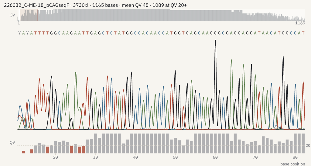
openreadout plot draws the same read as a figure, with a title, annotations and other panels
beside it: {"data": {"file": "read.ab1"}, "x": {"range": [80, 160]}} draws bases 80 to 160. In
the SVG each base’s trace, the base calls and the quality bars are a group of their own
(data-series="A", "base calls", "quality").
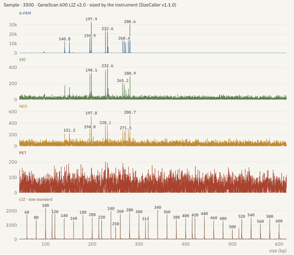
A fragment-analysis run is drawn as electropherograms on a base-pair axis, one panel per dye with
its tallest peaks labelled by size, and the size standard at the bottom with each fragment
labelled by its length. --x-range 180:300 zooms.
Examples
openreadout info read.ab1 # sample, instrument, read length, mean qualityopenreadout table read.ab1 # base calls: position, base, quality, scanopenreadout export read.ab1 # read.fastq (Phred+33)openreadout analyze peaks run.fsa --trace 0 --channel 1 # peaks of dye 1, sized in bpopenreadout table run.fsa --table 0 # the size standard's matched fragmentsHow this reader was derived, file by file: provenance log.