Pictures straight from raw files
Every picture on this page was drawn by the openreadout binary from a public instrument file, with no vendor software and no
plotting library. These are the pictures your agent sees and shows you, and the commands and specs under each one make them again.
Previews
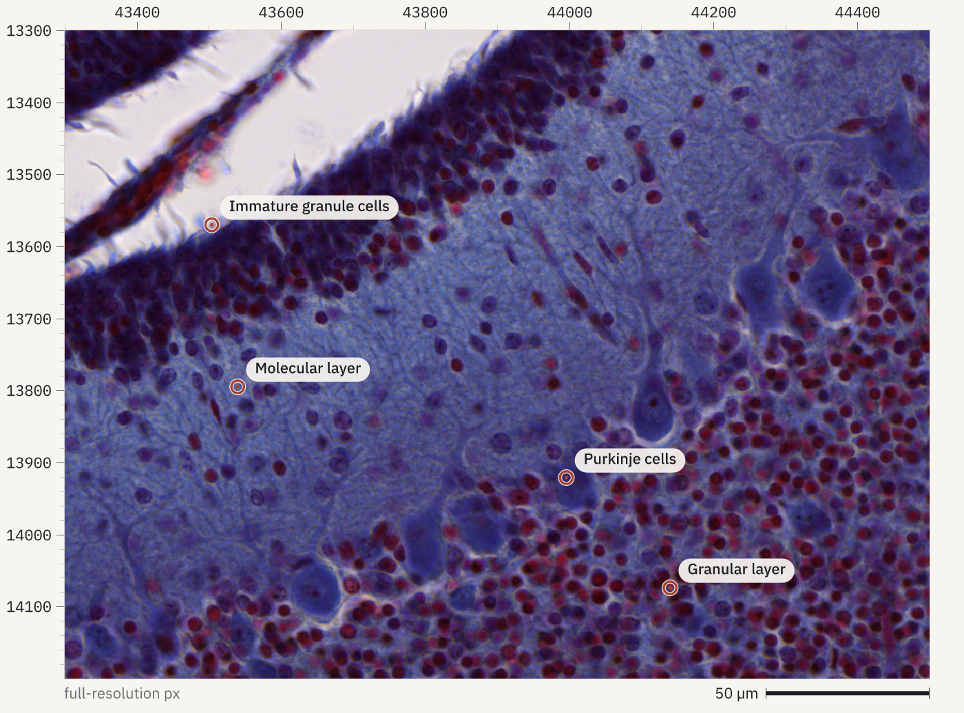
A preview is a quick look at one thing in a file: an image plane, a trace, a spectrum, a plate or a cytometry run. Images come with rulers in file pixels, so an agent can read positions off the picture, zoom into a region and put labelled marks where it sees something. Ask for one with openreadout preview, the agent tool openreadout_preview or File.preview() in Python.
How it was made
openreadout preview zenodo10577621-Young-mouse.czi --region 43300,13300,1200,900 --level 0 --max-size 1400 --annotate '[{"type":"point","x":43504,"y":13570,"label":"Immature granule cells"},{"type":"point","x":43540,"y":13795,"label":"Molecular layer"},{"type":"point","x":43996,"y":13921,"label":"Purkinje cells"},{"type":"point","x":44140,"y":14074,"label":"Granular layer"}]' -o slide-fold.png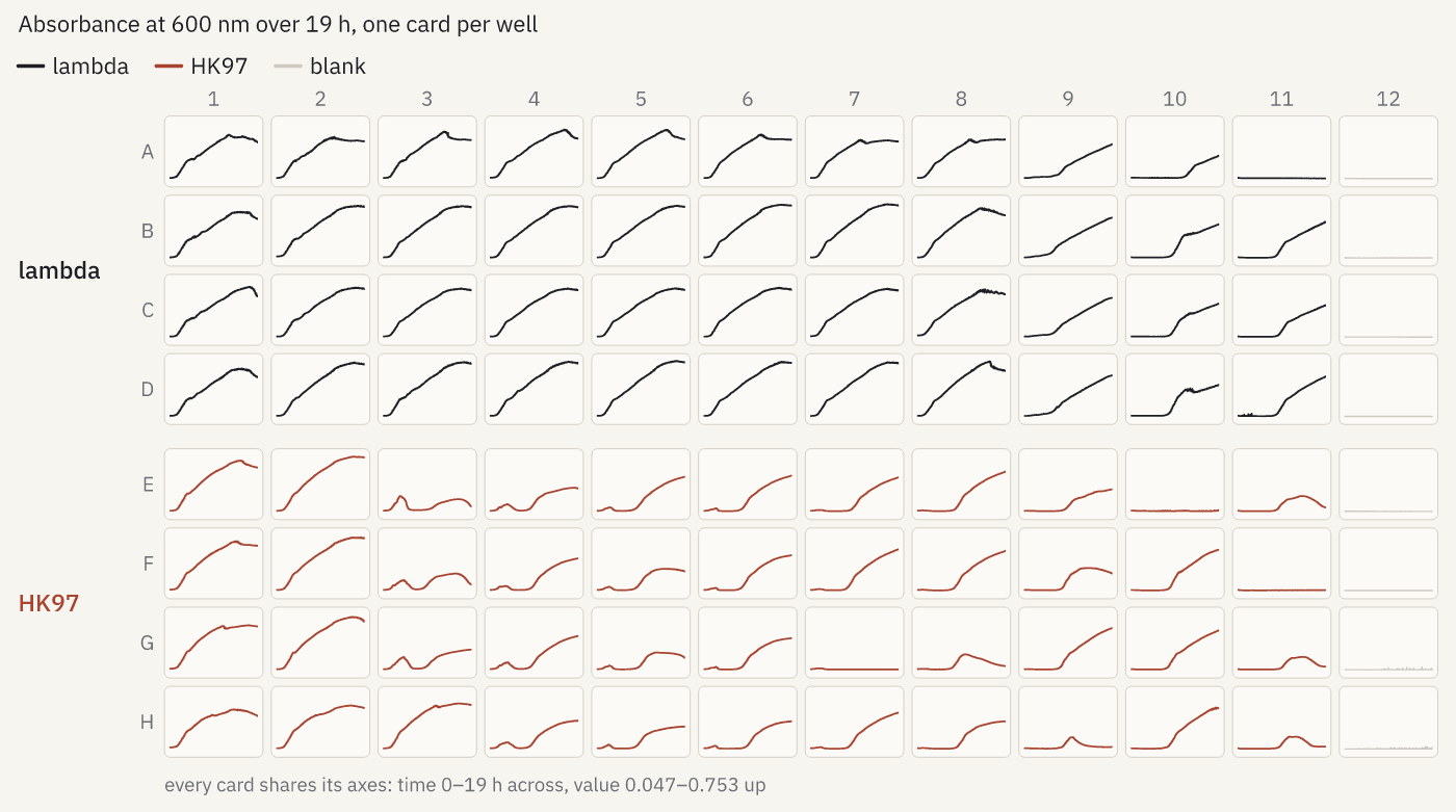
How it was made
openreadout preview softmax5-kinetic-phage-120308b.pda --max-size 1400 -o growth-grid.png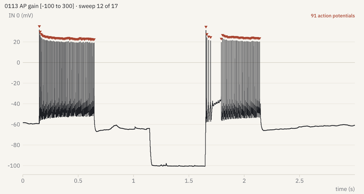
--marks spikes.
How it was made
openreadout preview pyabf-2019-07-24-0055-fsi.abf --sweep 12 --marks spikes --max-size 1200 -o spikes.png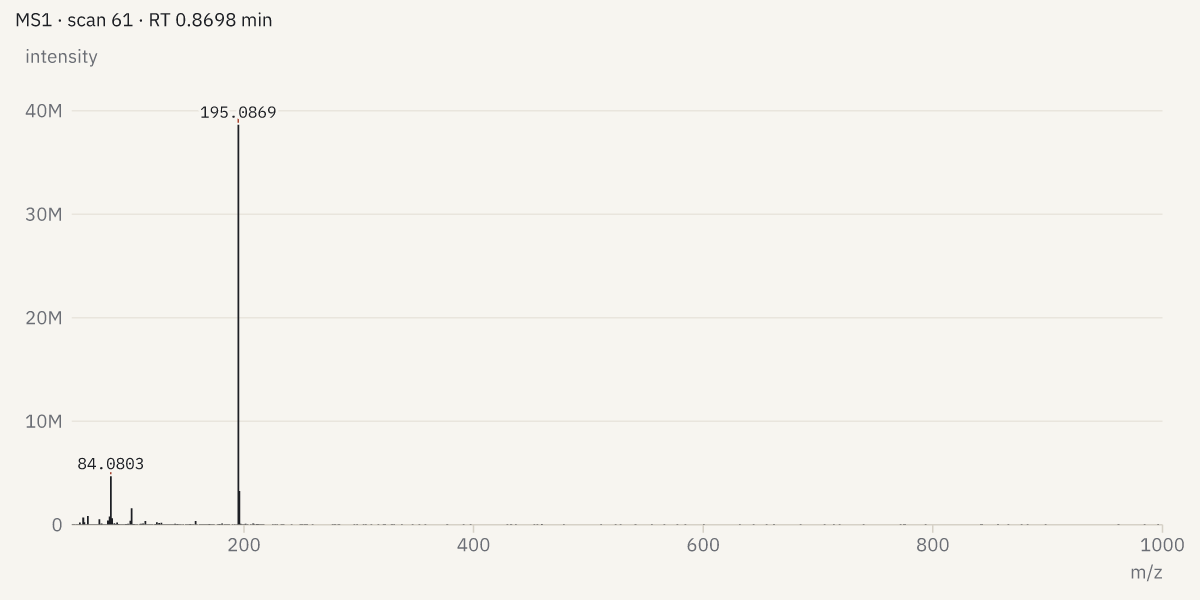
How it was made
openreadout preview mtbls20-caffeine-pos.mzML --spectrum 60 --max-size 1200 -o spectrum.png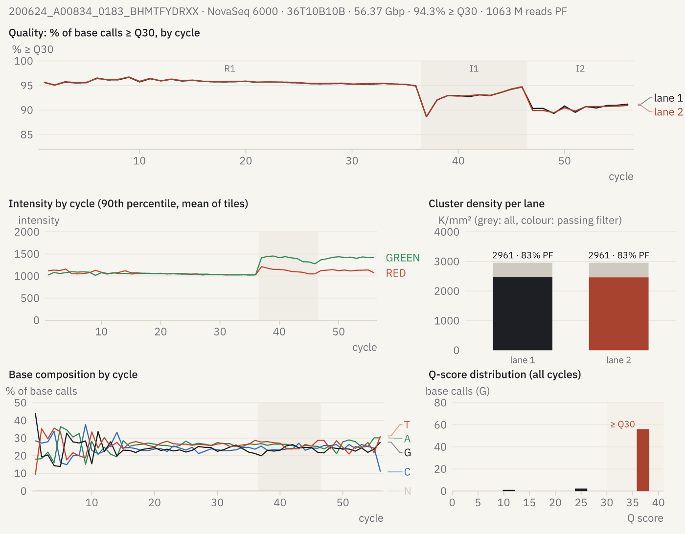
How it was made
openreadout preview 200624_A00834_0183_BHMTFYDRXX --max-size 1400 -o run-quality.png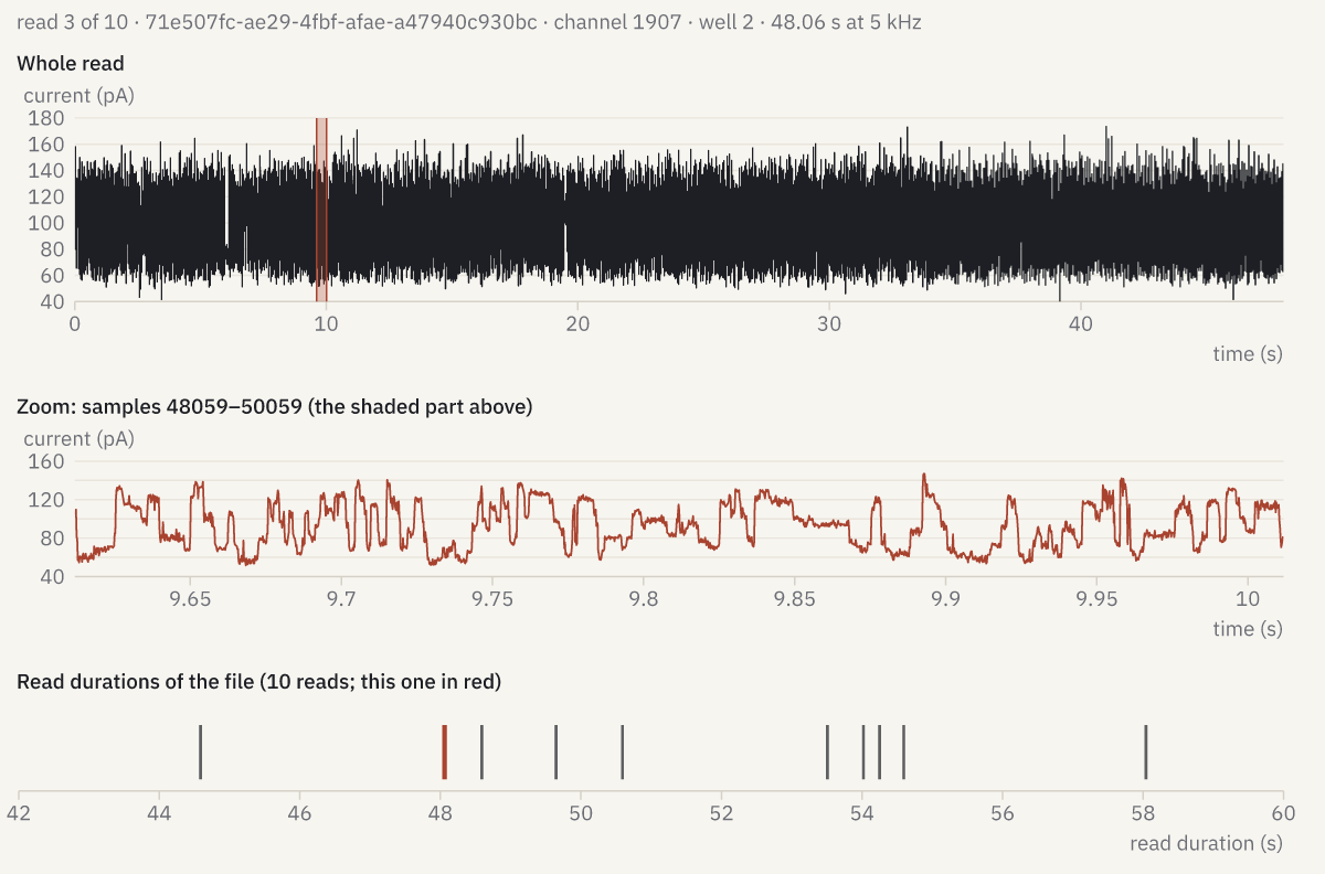
How it was made
openreadout preview seq-pod5-hg002-10reads.pod5 --sweep 3 --max-size 1200 -o squiggle.png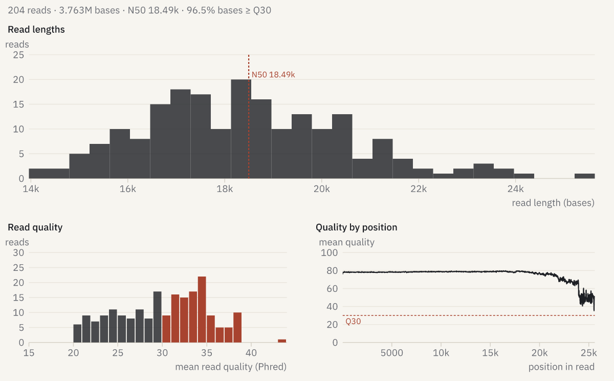
How it was made
openreadout preview seq-fastq-pacbio-hifi.fastq.gz --max-size 1200 -o read-lengths.png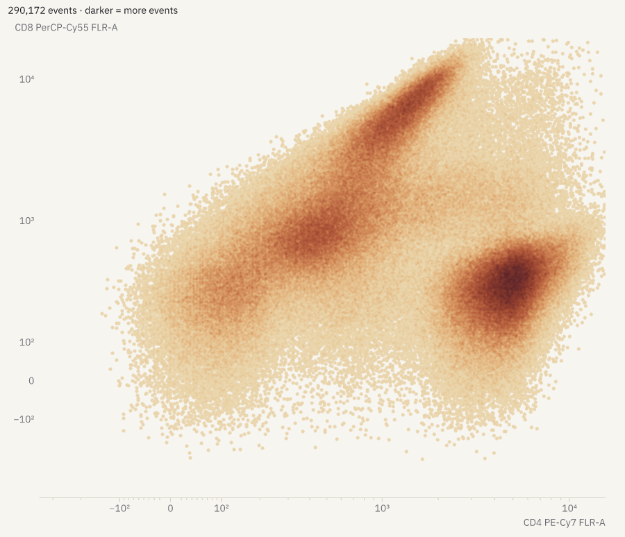
How it was made
openreadout preview flowkit-8c-e01.fcs --column 'CD4 PE-Cy7 FLR-A' --column 'CD8 PerCP-Cy55 FLR-A' --max-size 900 -o flow-density.png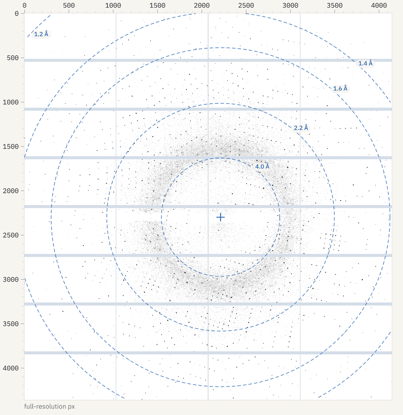
How it was made
openreadout preview Therm_6_1_master.h5 --max-size 1400 -o diffraction.png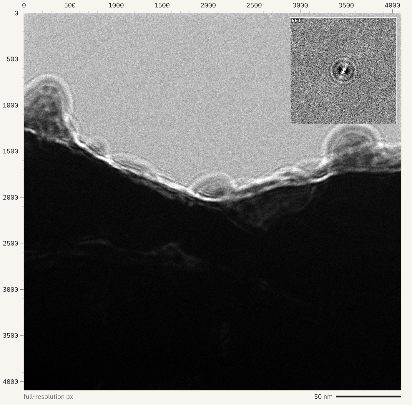
How it was made
openreadout preview empiar13509-glacios_00817_1-7.eer --sum t --fft --max-size 1400 -o cryoem-micrograph.png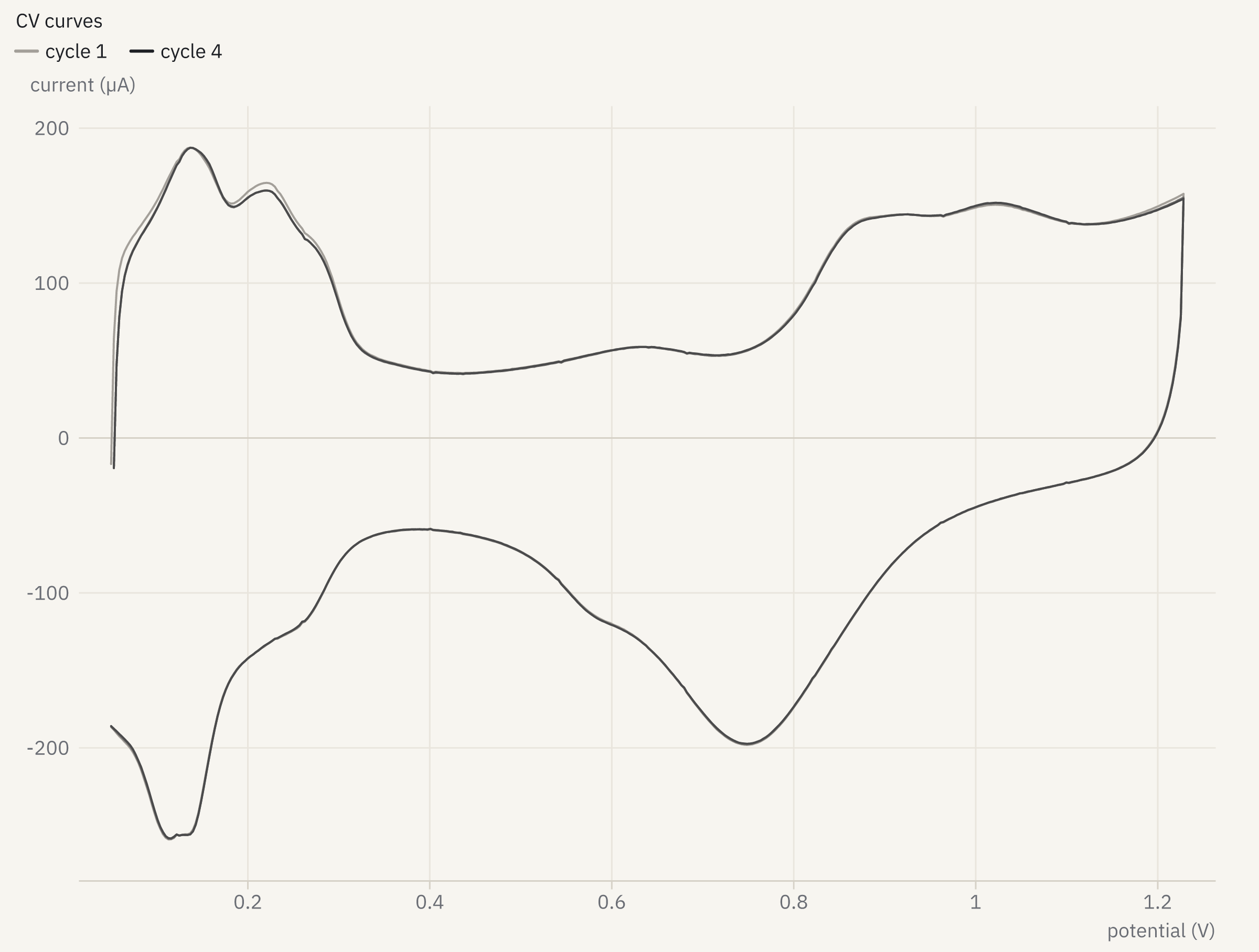
How it was made
openreadout preview echem-zenodo7245929-rde-cv-dimethyl.DTA --trace 1 --max-size 1200 --scale 2 -o cyclic-voltammogram.pngLight microscopy
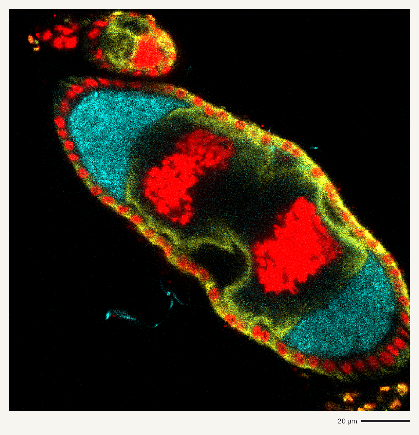
Previews of confocal, light-sheet and high-content images in seven file formats. Channels are overlaid, and the scale bar comes from the pixel size stored in the file.
How it was made
openreadout preview zenodo8298760-Orb-Vas-PI-1-mei-P26-1-uninf-4-5d-211024.lif --composite --axes scale-bar --max-size 1400 -o drosophila-egg-chamber.png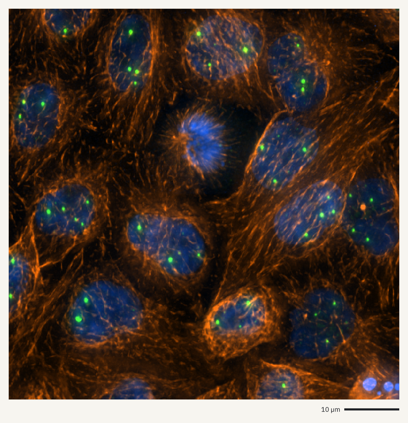
How it was made
openreadout preview 090829_1_HeLa_siCTL_coilin_ATUB01_01_R3D_D3D.dv --composite --mip z --region 32,32,448,448 --axes scale-bar --max-size 1400 -o hela-cajal-bodies.png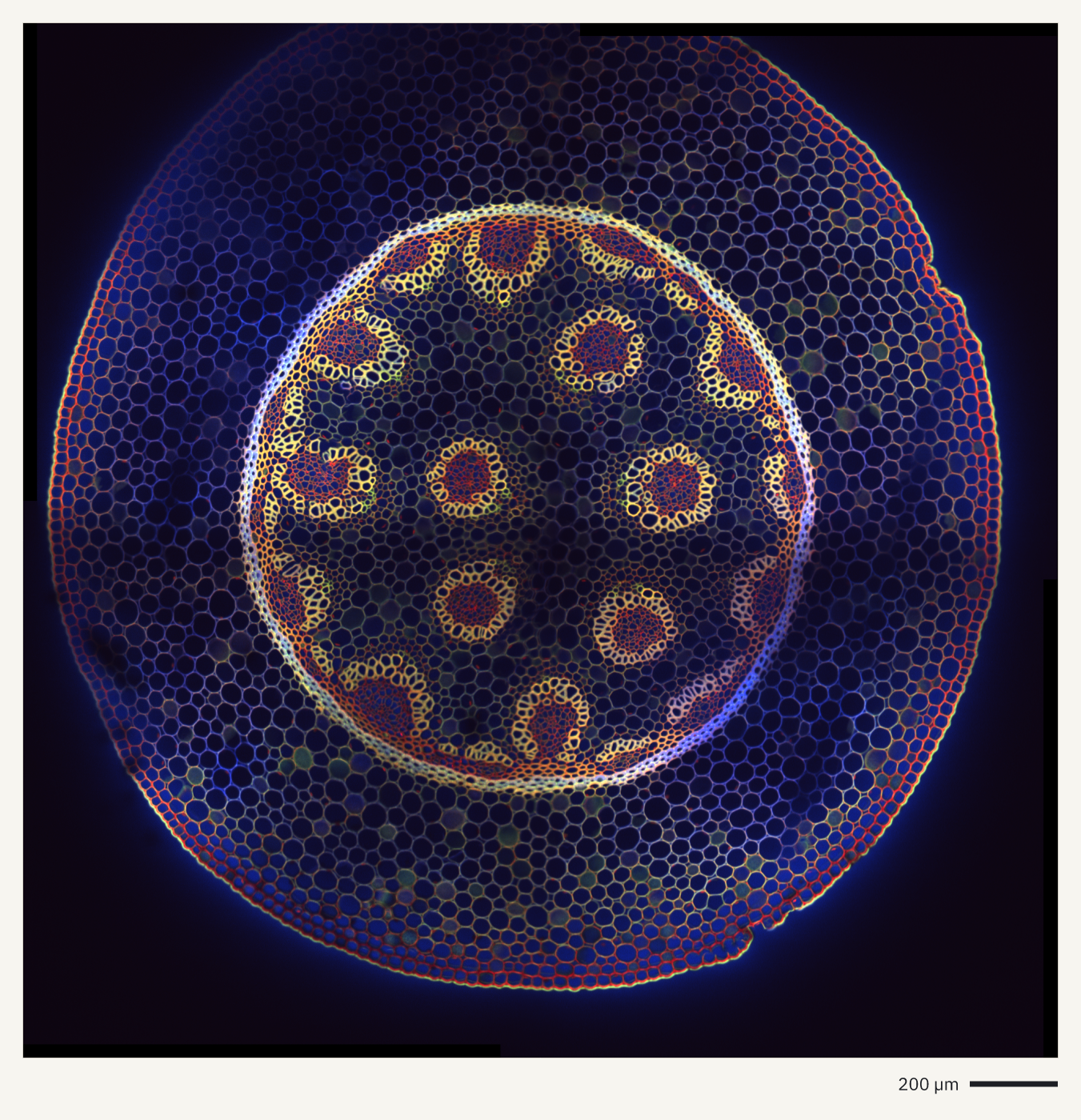
How it was made
openreadout preview Convallaria_3C_1T_2x2grid_confocal.ims --composite --axes scale-bar --max-size 1400 -o convallaria-root.png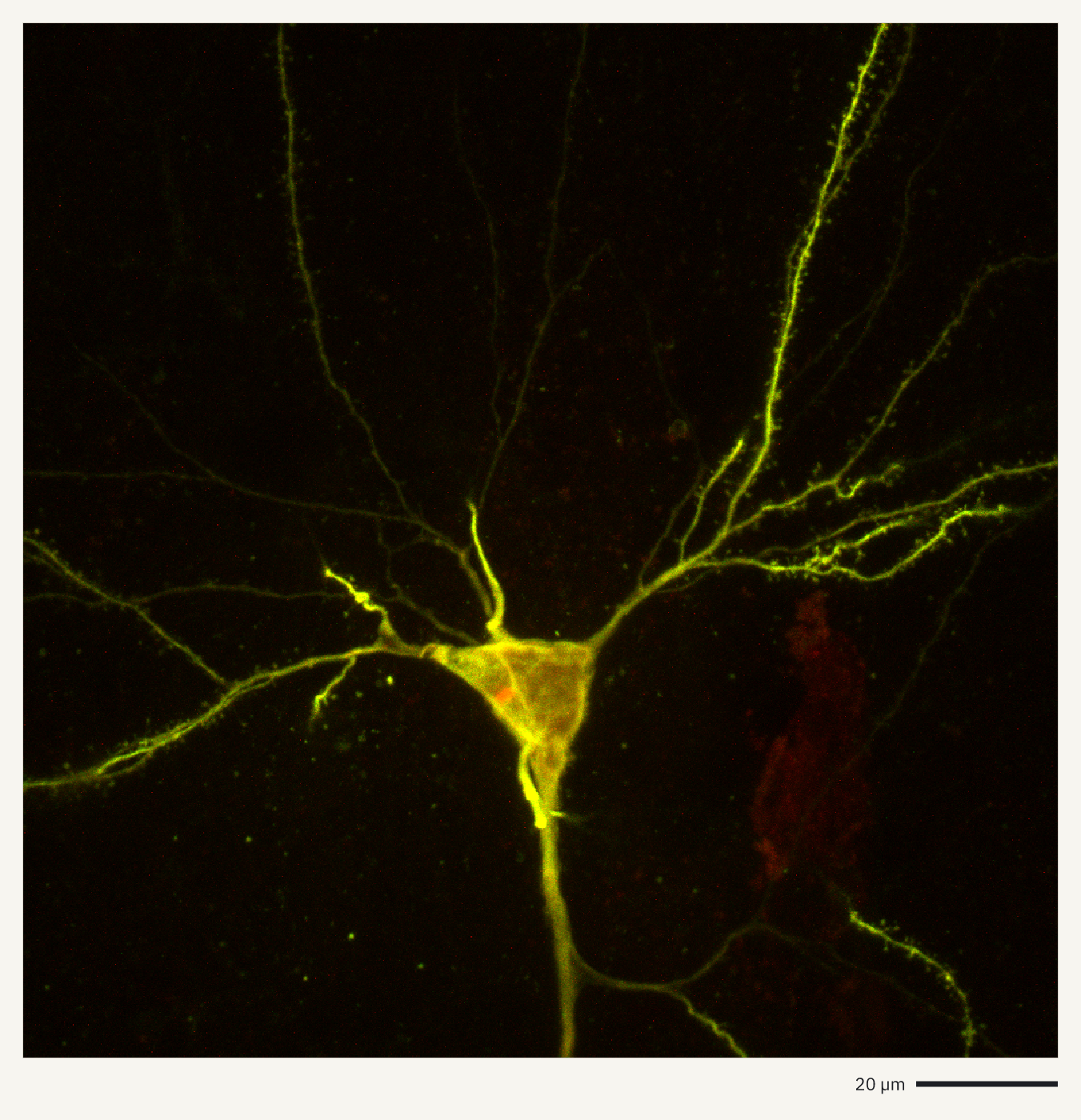
How it was made
openreadout preview zenodo14235726-performanceTestImage.ims --composite --mip z --axes scale-bar --max-size 1400 -o neuron-imaris.png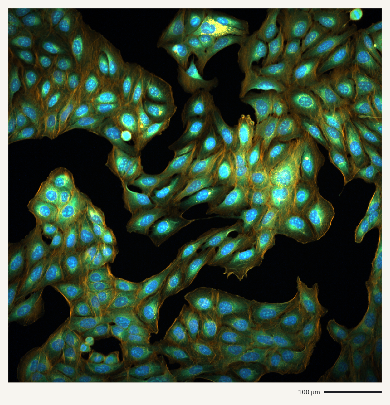
How it was made
openreadout preview MeasurementData.mlf --select c=0,1,3 --mip z --axes scale-bar --max-size 1400 -o cell-painting-cv8000.png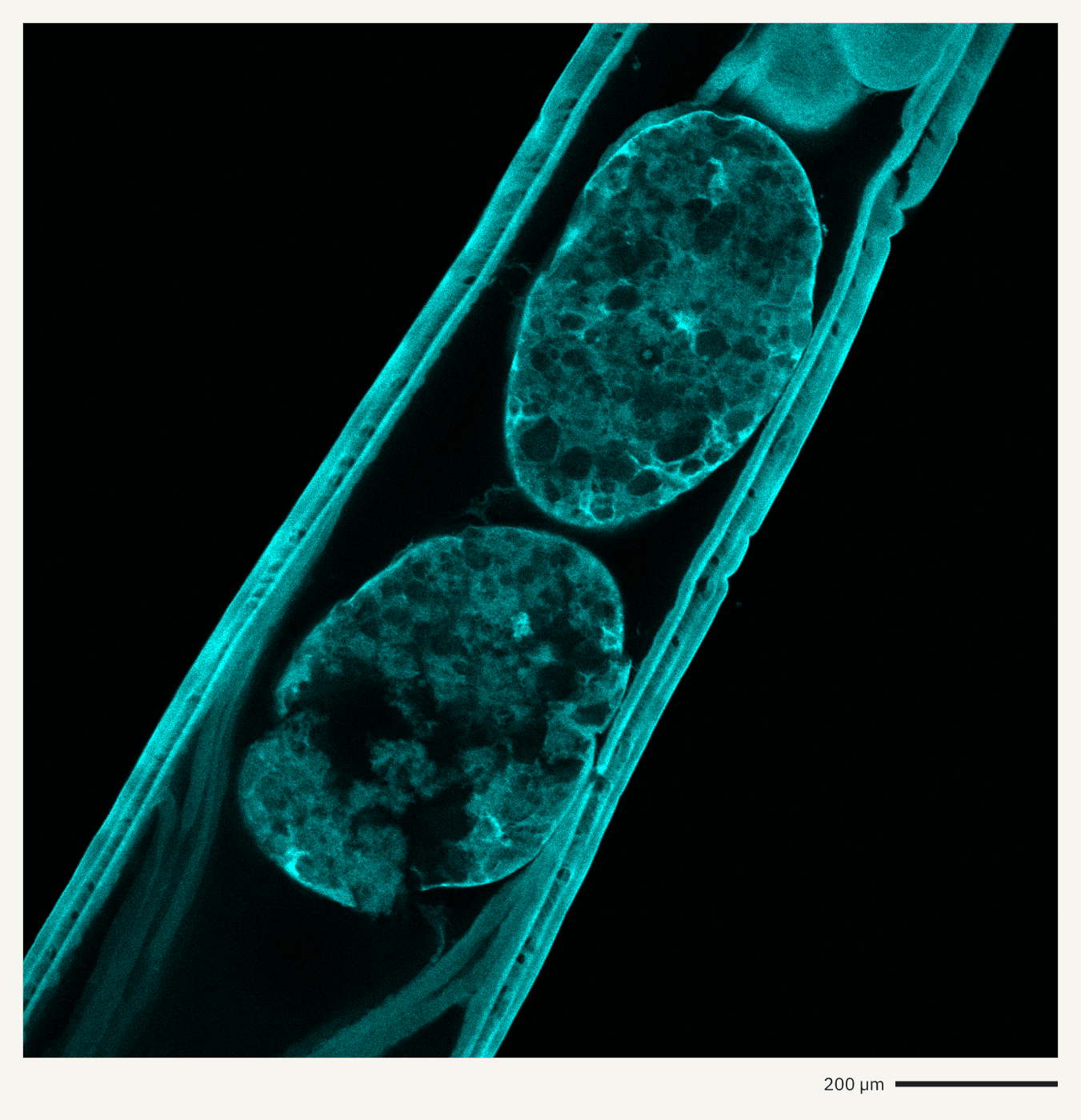
How it was made
openreadout preview figshare22922456-E3-6-testes.oir --composite --axes scale-bar --max-size 1400 -o testes-oir.png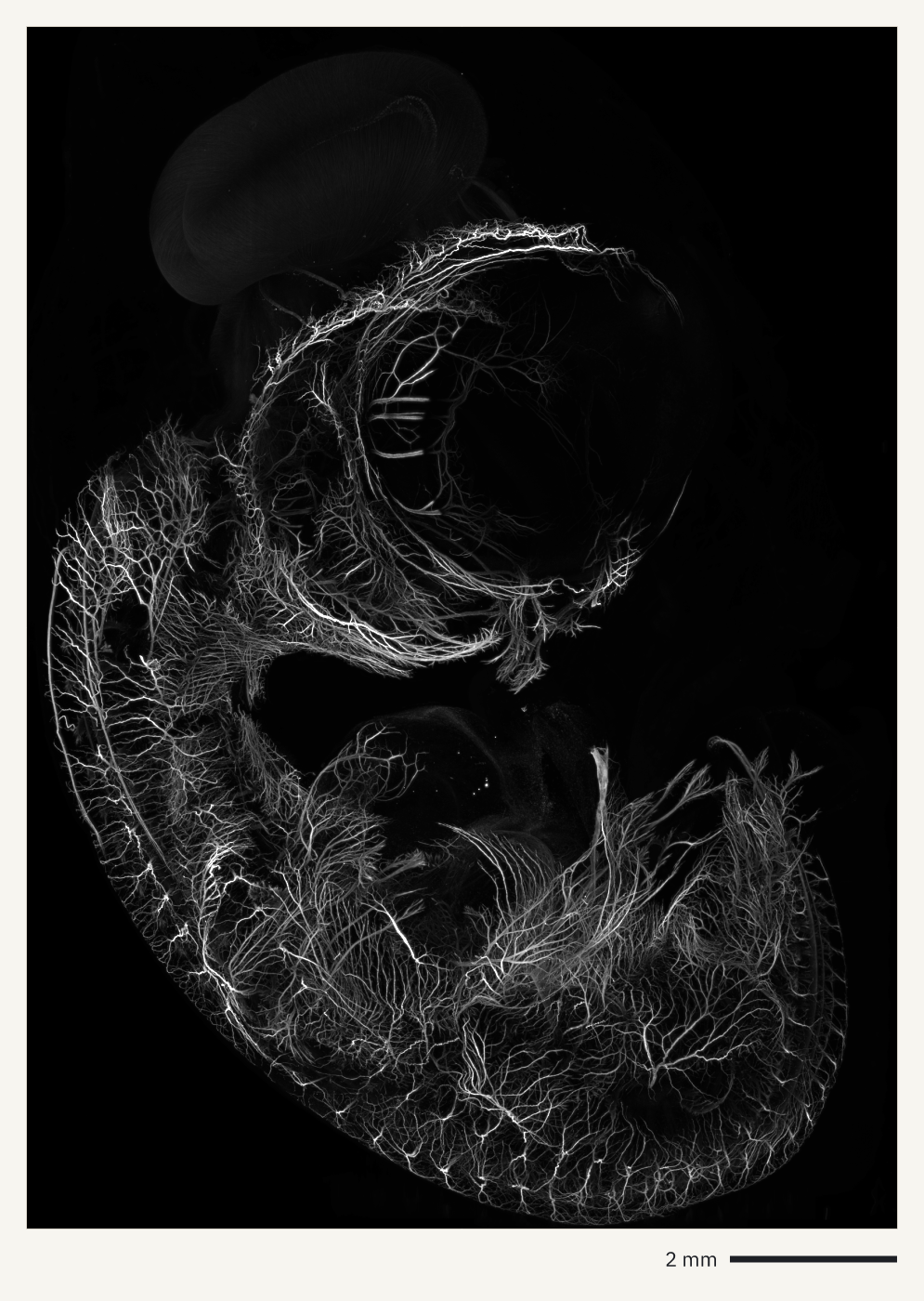
How it was made
openreadout preview ExpD_chicken_embryo_MIP.ome.zarr --axes scale-bar --max-size 1400 -o chicken-embryo-mesospim.png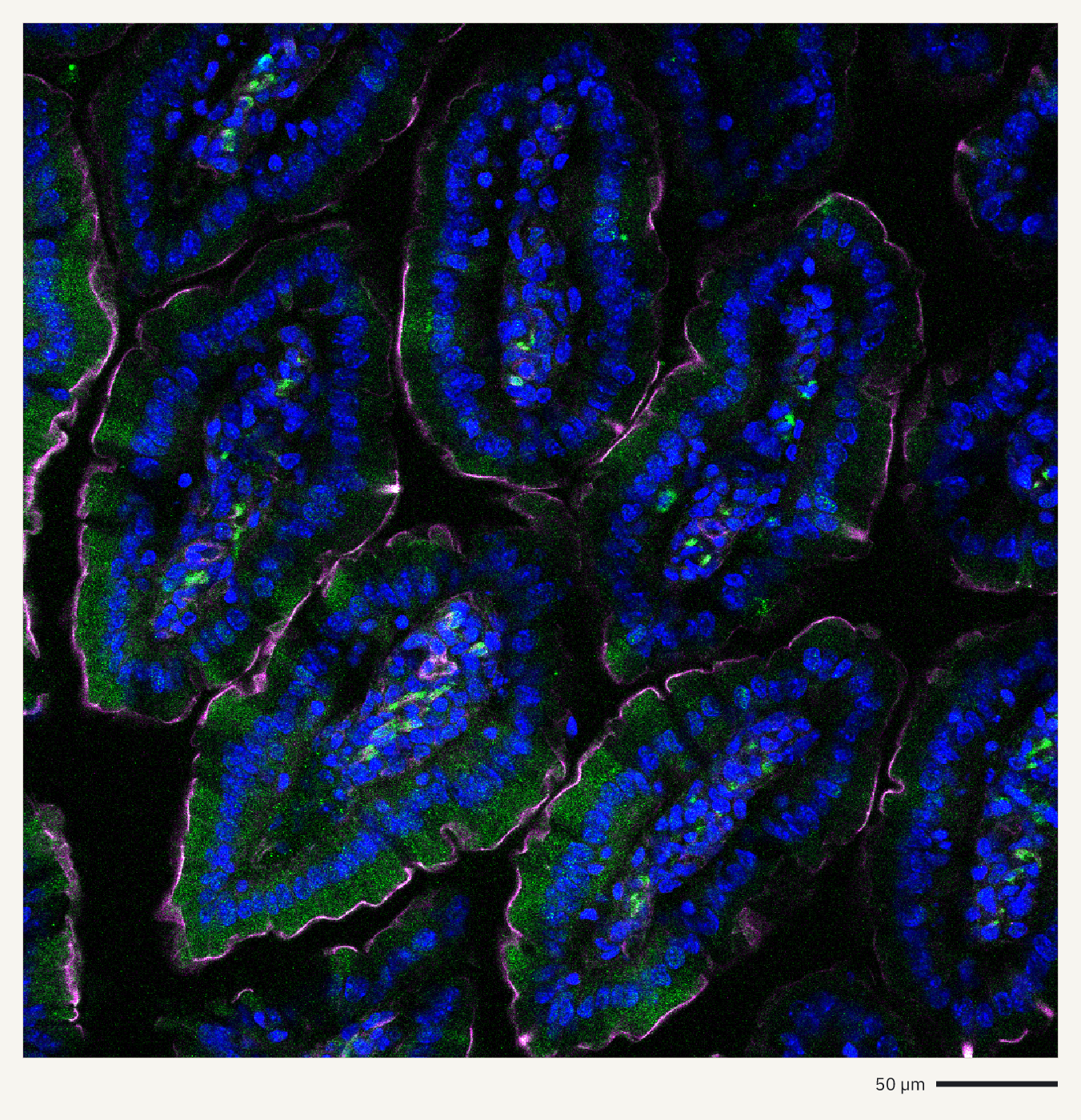
How it was made
openreadout preview zenodo5823010-inflammasome.czi --composite --axes scale-bar --max-size 1400 -o intestine-villi-lsm710.pngElectron microscopy and other imaging
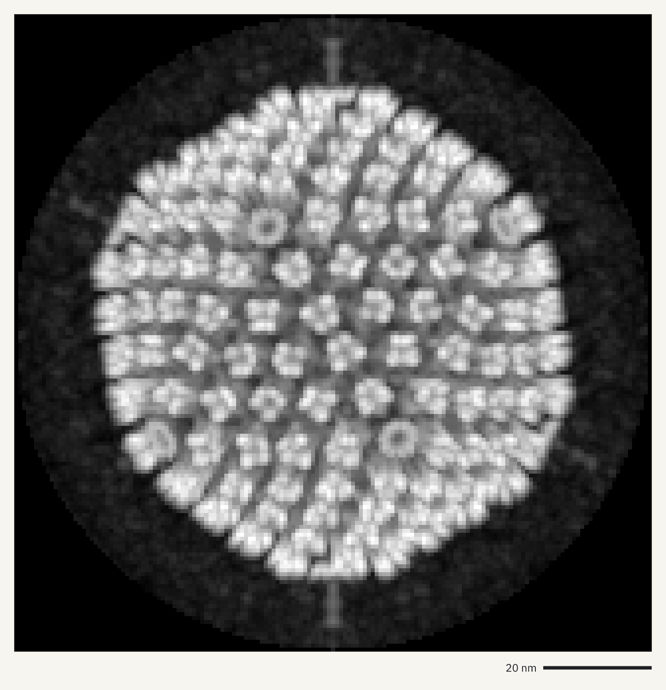
Previews of electron micrographs, a diffraction pattern, a density map, a tomogram and an MRI scan. --sum adds up frames and --mip projects a stack.
How it was made
openreadout preview emdb-emd-1016.map.gz --mip z --axes scale-bar --max-size 1400 -o virus-capsid-map.png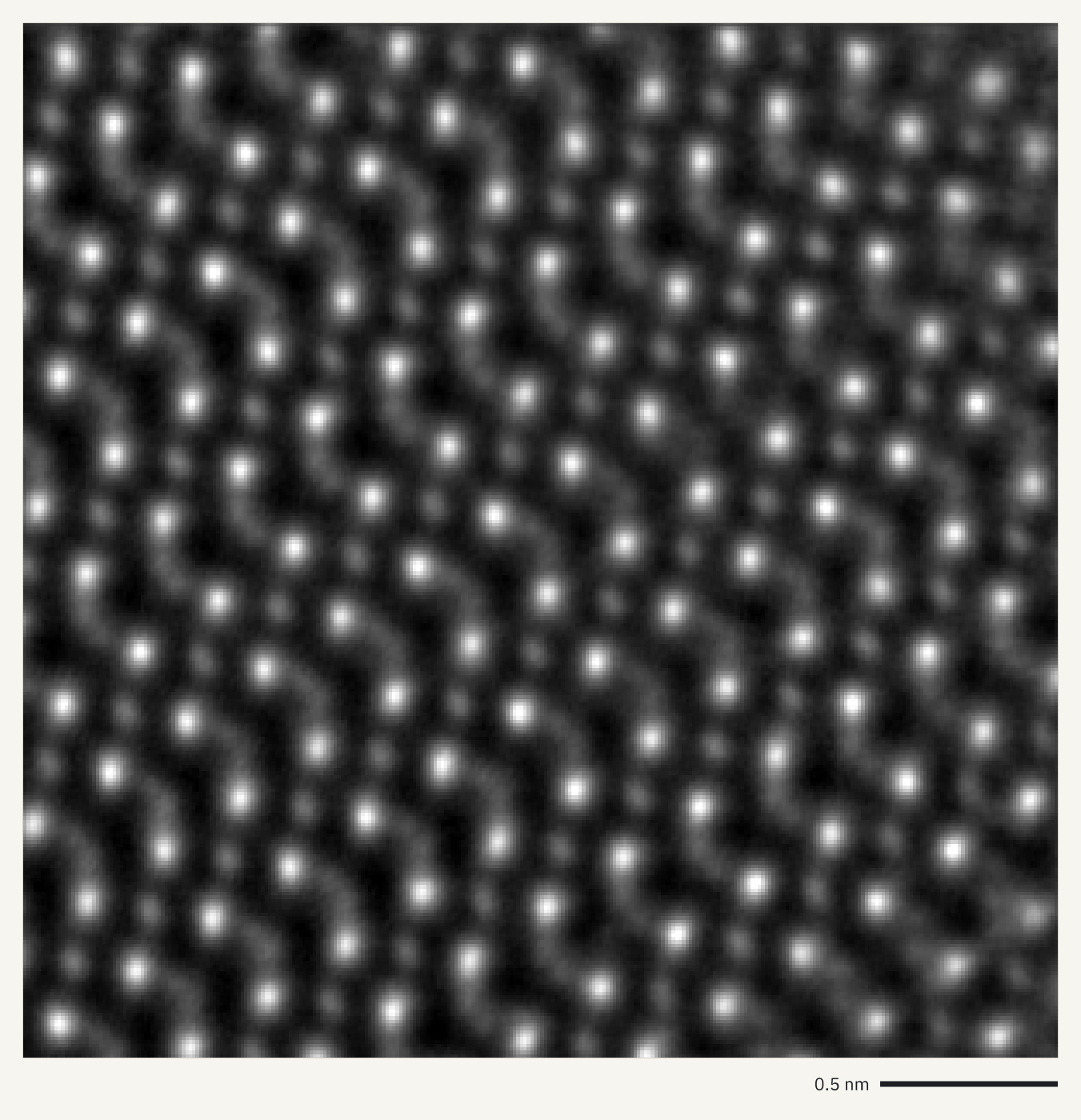
How it was made
openreadout preview zenodo18373896-hzo-ptycho.dm3 --sum t --axes scale-bar --max-size 1400 -o hzo-ptychography.png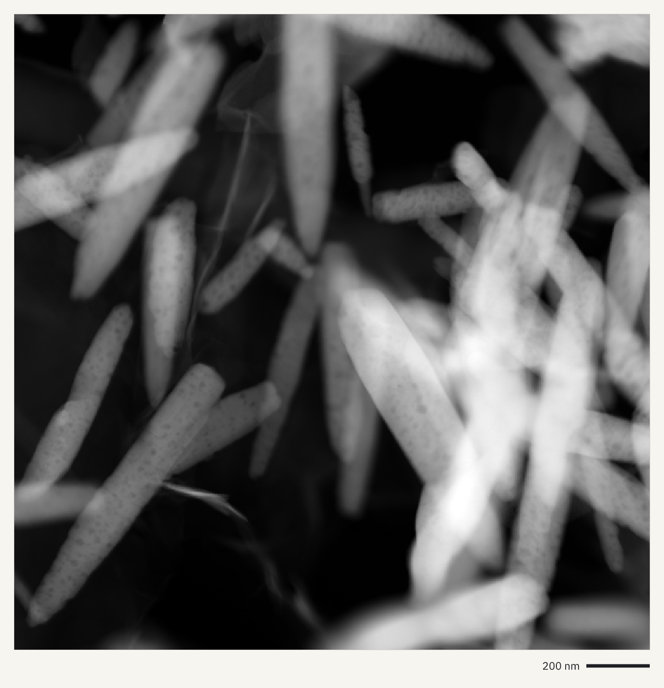
How it was made
openreadout preview zenodo10848941-go-zno.dm4 --axes scale-bar --max-size 1400 -o zno-nanorods.png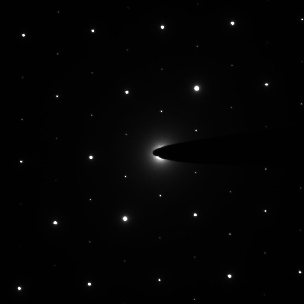
How it was made
openreadout preview zenodo13821437-Figure-2e.dm4 --axes none --max-size 1400 -o saed-spot-pattern.png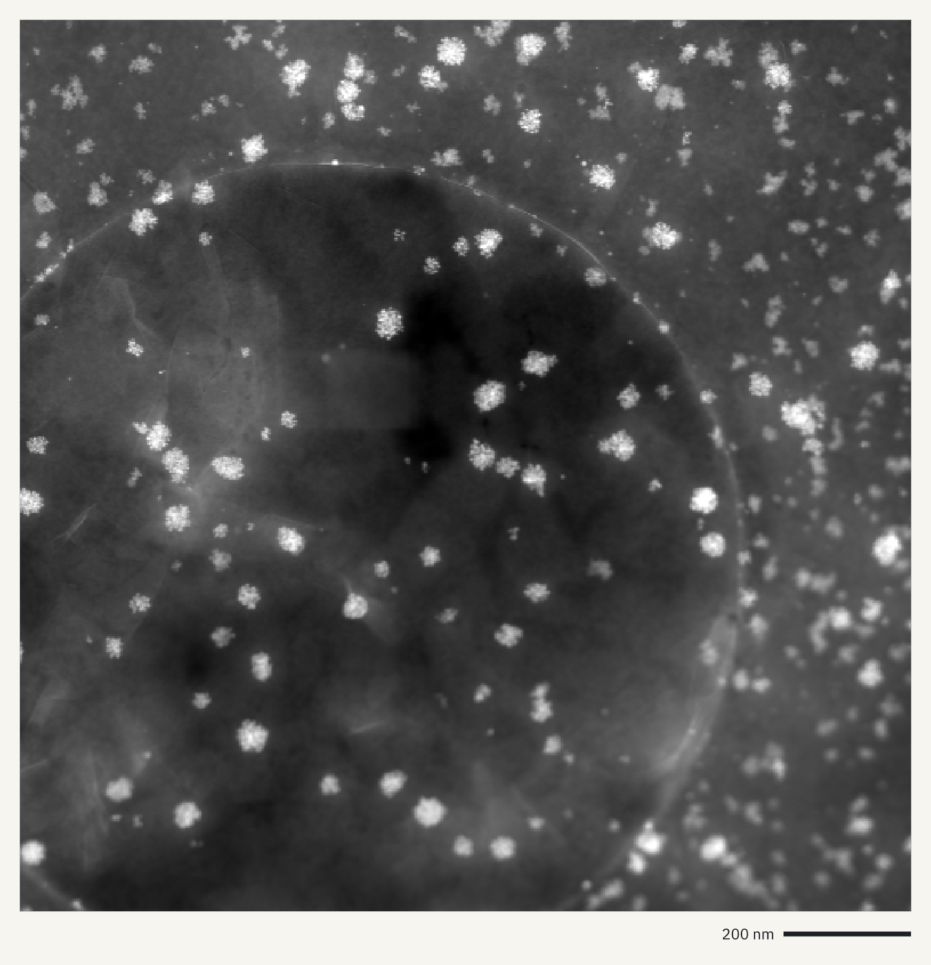
How it was made
openreadout preview zenodo20131712-0017-SI-Nano-1.4um.emd --sum t --axes scale-bar --max-size 1400 -o nanoparticles-haadf.png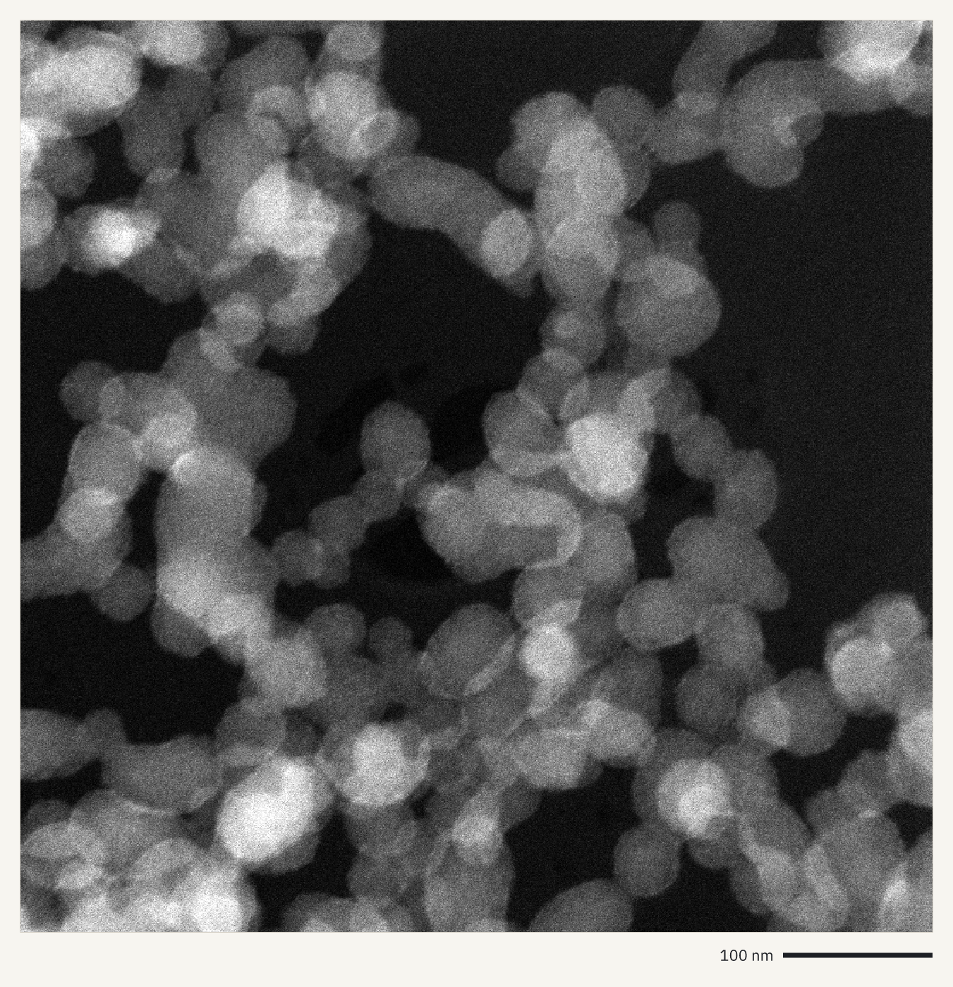
How it was made
openreadout preview zenodo17463176-Fig_b1_1.ser --axes scale-bar --max-size 1400 -o silica-particles-tem.png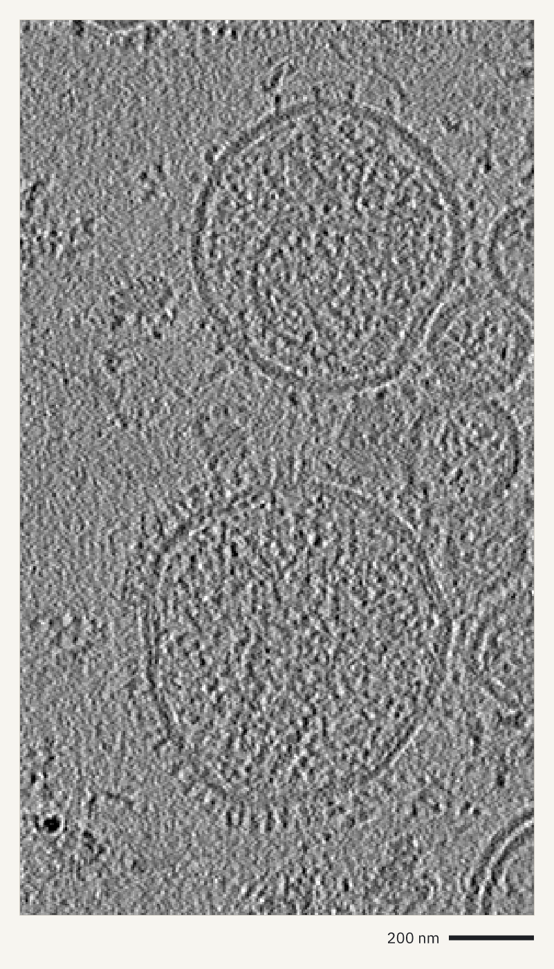
How it was made
openreadout preview zenodo10526574-IPPK-TS08-rec.rec --axes scale-bar --max-size 1400 -o cryo-et-tomogram.png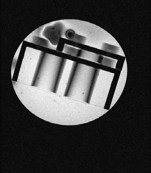
How it was made
openreadout preview 20210128_122257_LEGO_PHANTOM_API_TEST_1_1 --image 14 --axes none --max-size 1400 -o lego-phantom-mri.pngFigures
A figure is a finished plot of data from one or more files, described in a few lines of JSON: which file and which trace, wells or parameters, and how to arrange them. OpenReadout picks the chart, the axes, the units and the labels. Draw one with openreadout plot, the agent tool openreadout_plot or openreadout.plot() in Python.
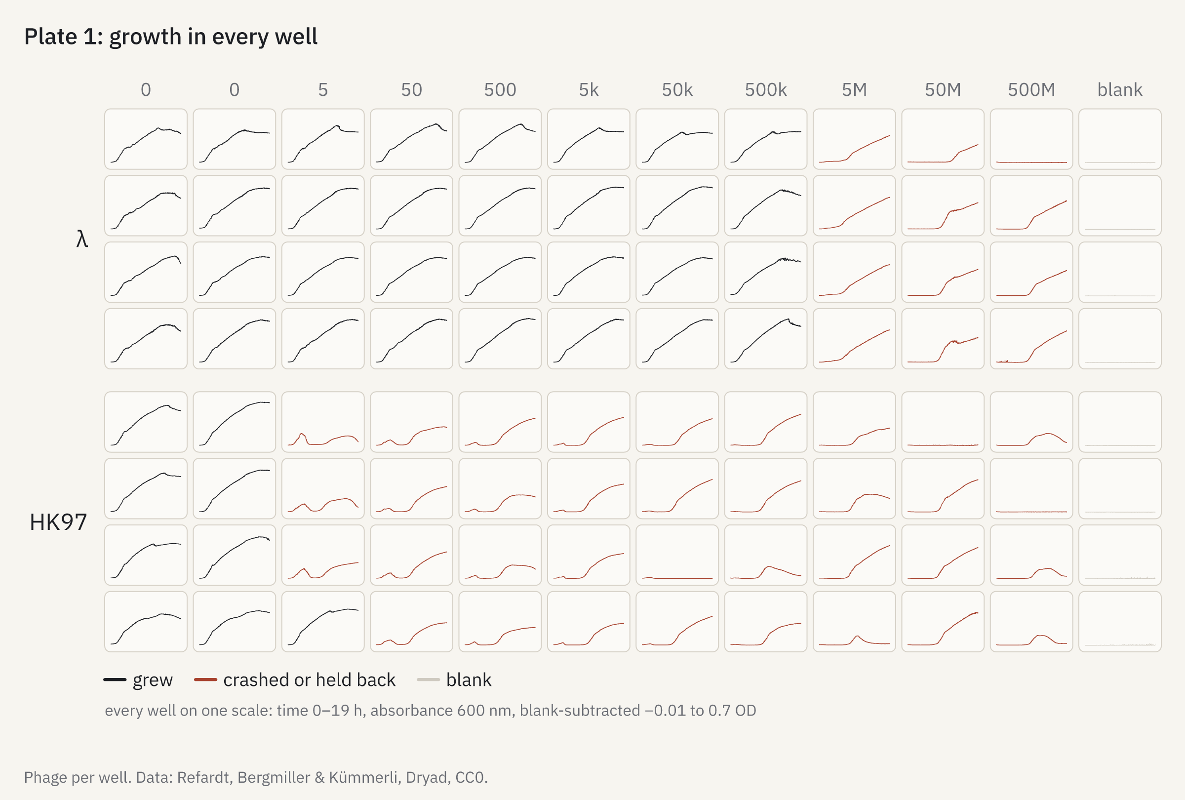
How it was made
openreadout plot plate-grid.json -o plate-grid.png{
"title": "Plate 1: growth in every well",
"data": {
"file": "softmax5-kinetic-phage-120308b.pda",
"subtract": "blank",
"color_by": {
"at": 6,
"below": 0.1,
"label": "crashed or held back",
"else": "grew"
}
},
"facet": "plate",
"row_labels": [
"λ",
"HK97"
],
"column_labels": [
"0",
"0",
"5",
"50",
"500",
"5k",
"50k",
"500k",
"5M",
"50M",
"500M",
"blank"
],
"caption": "Phage per well. Data: Refardt, Bergmiller & Kümmerli, Dryad, CC0."
}
How it was made
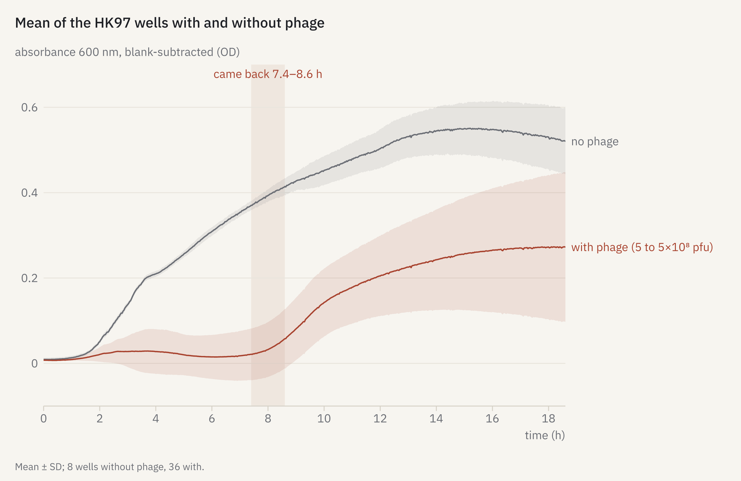
openreadout plot comeback.json -o comeback.png{
"title": "Mean of the HK97 wells with and without phage",
"data": [
{
"file": "softmax5-kinetic-phage-120308b.pda",
"wells": "E1:H2",
"by": "group",
"subtract": "blank",
"color": "muted",
"label": "no phage"
},
{
"file": "softmax5-kinetic-phage-120308b.pda",
"wells": "E3:H11",
"by": "group",
"subtract": "blank",
"color": "accent",
"label": "with phage (5 to 5×10⁸ pfu)"
}
],
"annotate": [
{
"type": "vband",
"x": 7.4,
"x2": 8.6,
"label": "came back 7.4–8.6 h"
}
],
"caption": "Mean ± SD; 8 wells without phage, 36 with."
}
How it was made
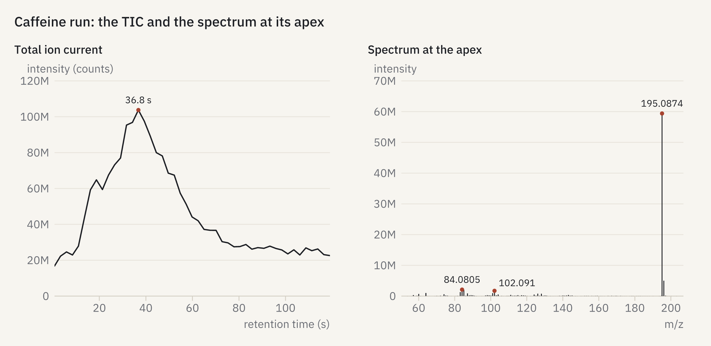
openreadout plot tic-spectrum.json -o tic-spectrum.png{
"title": "Caffeine run: the TIC and the spectrum at its apex",
"panels": [
{
"title": "Total ion current",
"data": {
"file": "mtbls20-caffeine-pos.mzML",
"peaks": 1
}
},
{
"title": "Spectrum at the apex",
"data": {
"file": "mtbls20-caffeine-pos.mzML",
"rt": "apex",
"peaks": 6
}
}
]
}
How it was made
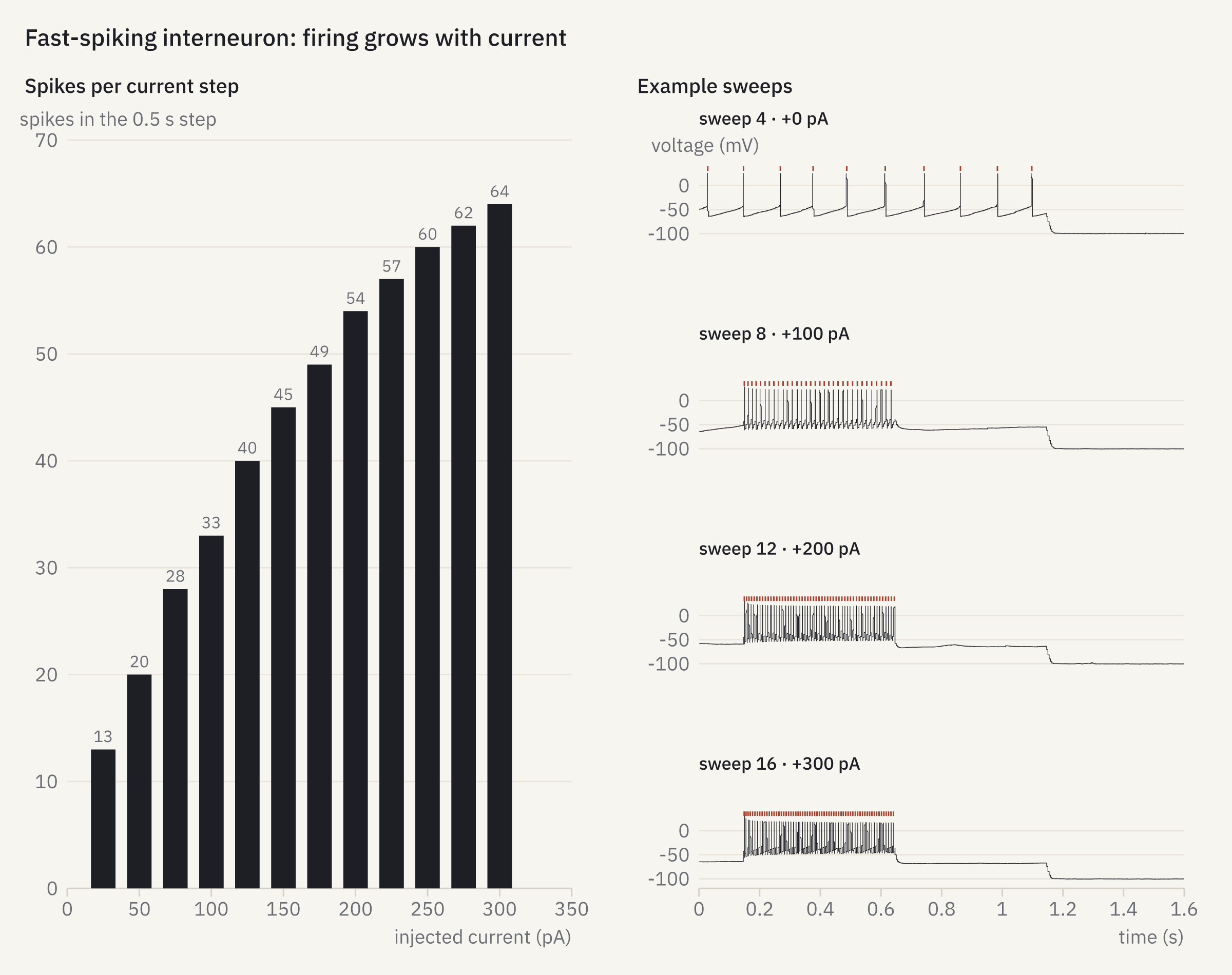
openreadout plot fi.json -o fi.png{
"title": "Fast-spiking interneuron: firing grows with current",
"panels": [
{
"title": "Spikes per current step",
"data": {
"file": "pyabf-2019-07-24-0055-fsi.abf",
"show": "fi",
"mark": "bars"
}
},
{
"title": "Example sweeps",
"data": {
"file": "pyabf-2019-07-24-0055-fsi.abf",
"show": "sweeps",
"sweep": [
4,
8,
12,
16
],
"spikes": true
},
"facet": "series",
"x": {
"range": [
0,
1.6
]
}
}
],
"columns": 2
}
How it was made
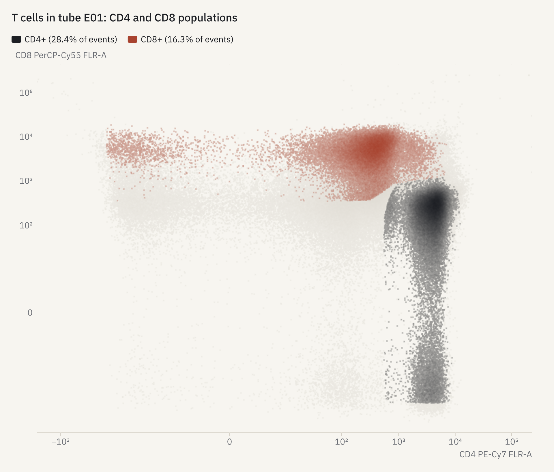
openreadout plot fcs-gates.json -o fcs-gates.png{
"title": "T cells in tube E01: CD4 and CD8 populations",
"data": {
"file": "flowkit-8c-e01.fcs",
"x": "CD4 PE-Cy7 FLR-A",
"y": "CD8 PerCP-Cy55 FLR-A",
"workspace": "flowkit-8c-ics.wsp",
"populations": [
"CD4+",
"CD8+"
]
}
}
How it was made
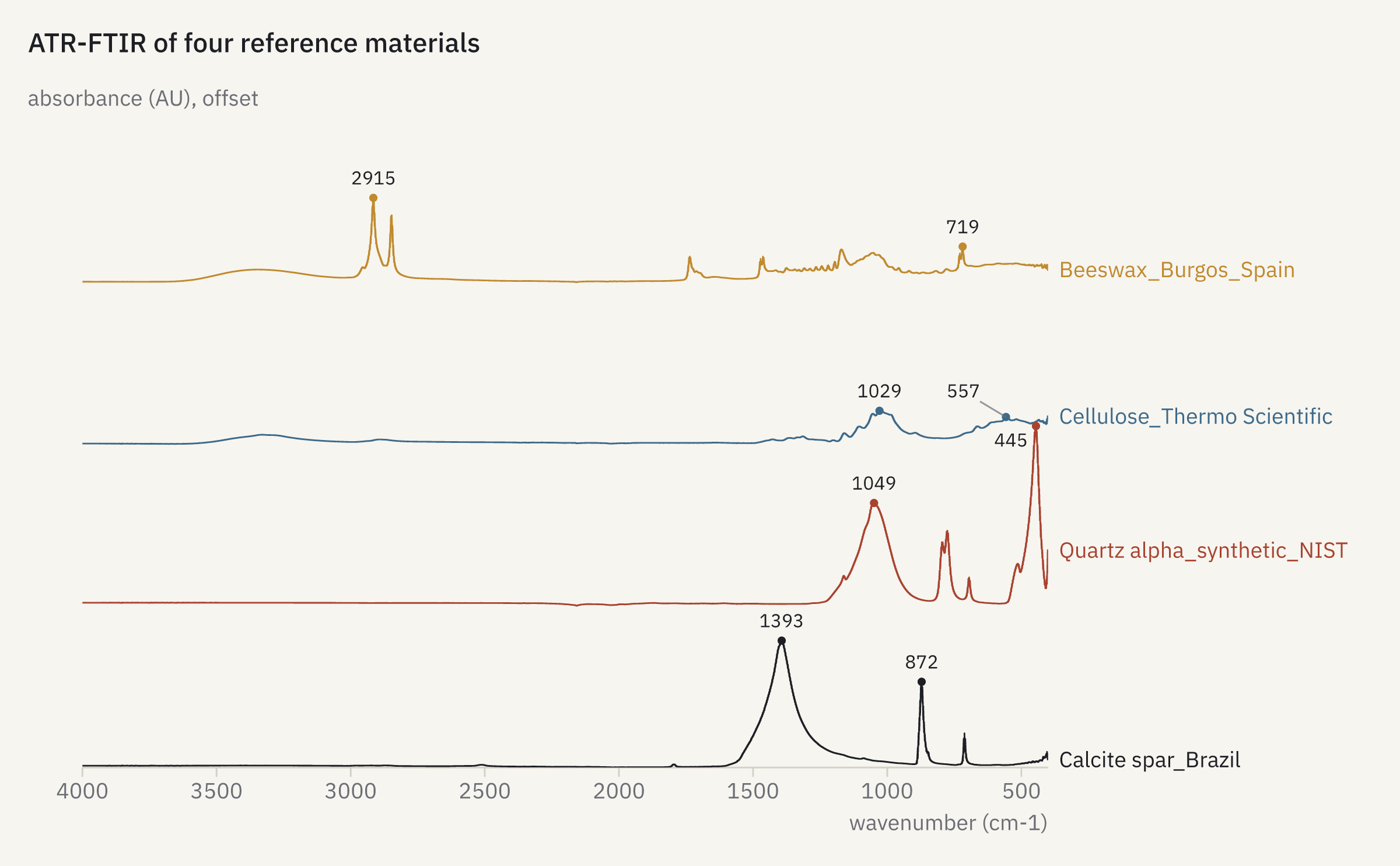
openreadout plot ir-overlay.json -o ir-overlay.png{
"title": "ATR-FTIR of four reference materials",
"data": {
"file": [
"Calcite spar_Brazil.SPA",
"Quartz alpha_synthetic_NIST.SPA",
"Cellulose_Thermo Scientific.SPA",
"Beeswax_Burgos_Spain.SPA"
],
"peaks": 2
},
"stack": 0.9
}
How it was made
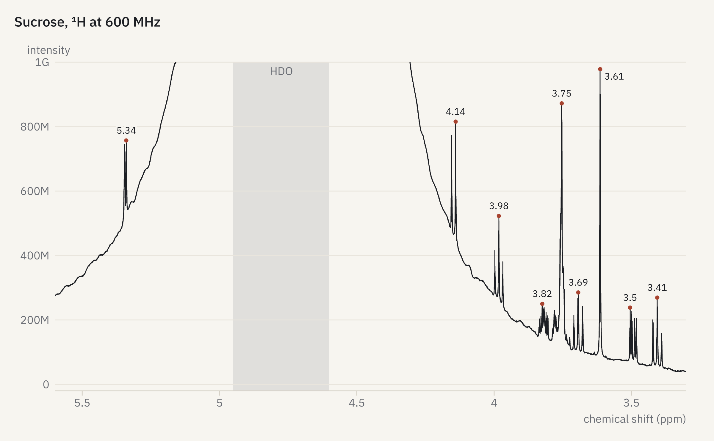
openreadout plot nmr.json -o nmr.png{
"title": "Sucrose, ¹H at 600 MHz",
"data": {
"file": "1",
"process": true,
"peaks": 10,
"x_range": [
3.3,
5.6
]
},
"y": {
"range": [
-20000000,
1000000000
]
},
"annotate": [
{
"type": "vband",
"x": 4.6,
"x2": 4.95,
"label": "HDO",
"color": "muted"
}
]
}
How it was made
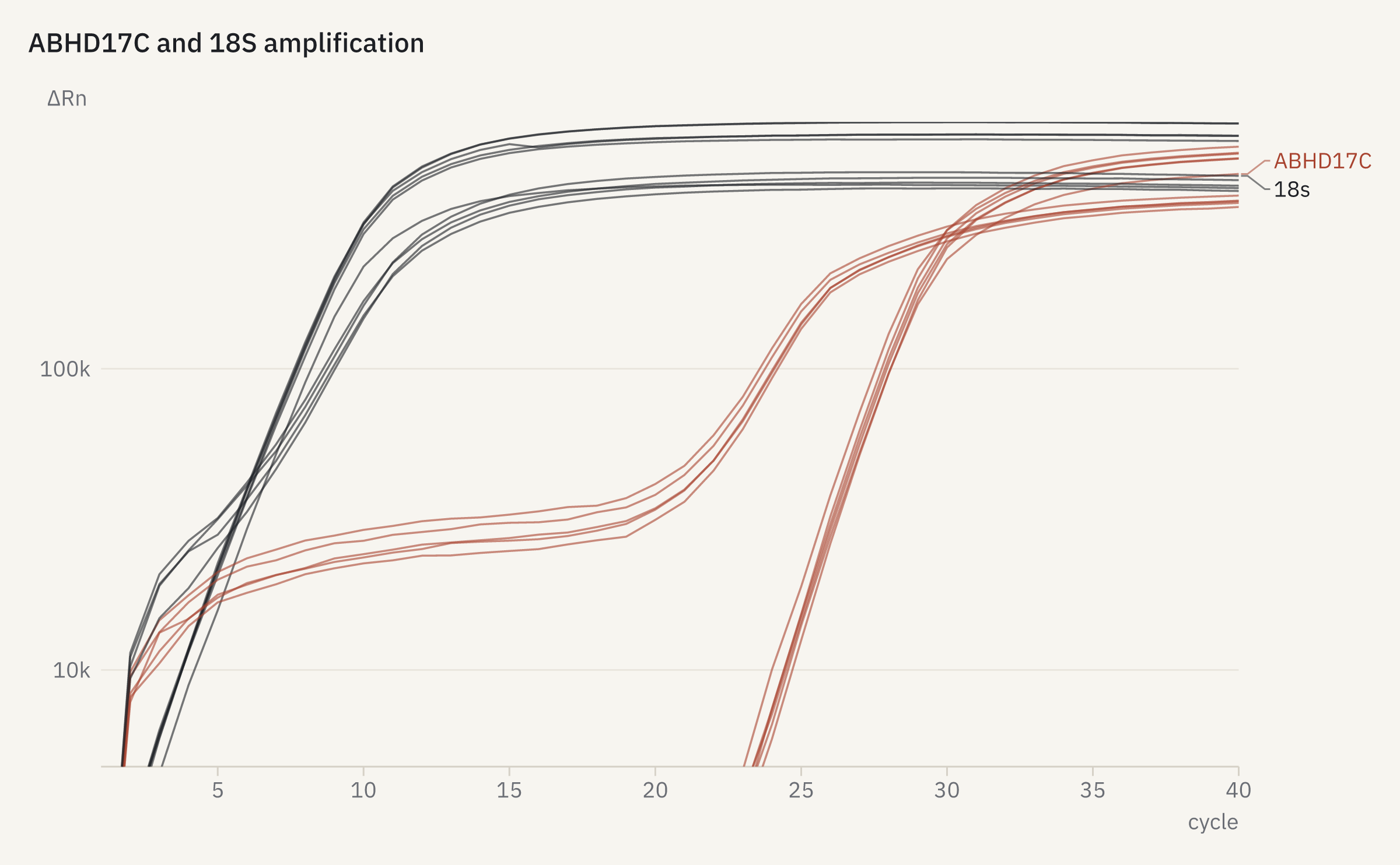
openreadout plot qpcr.json -o qpcr.png{
"title": "ABHD17C and 18S amplification",
"data": {
"file": "eds-7500-abhd17c-ddct.eds"
},
"y": {
"log": true
}
}
How it was made
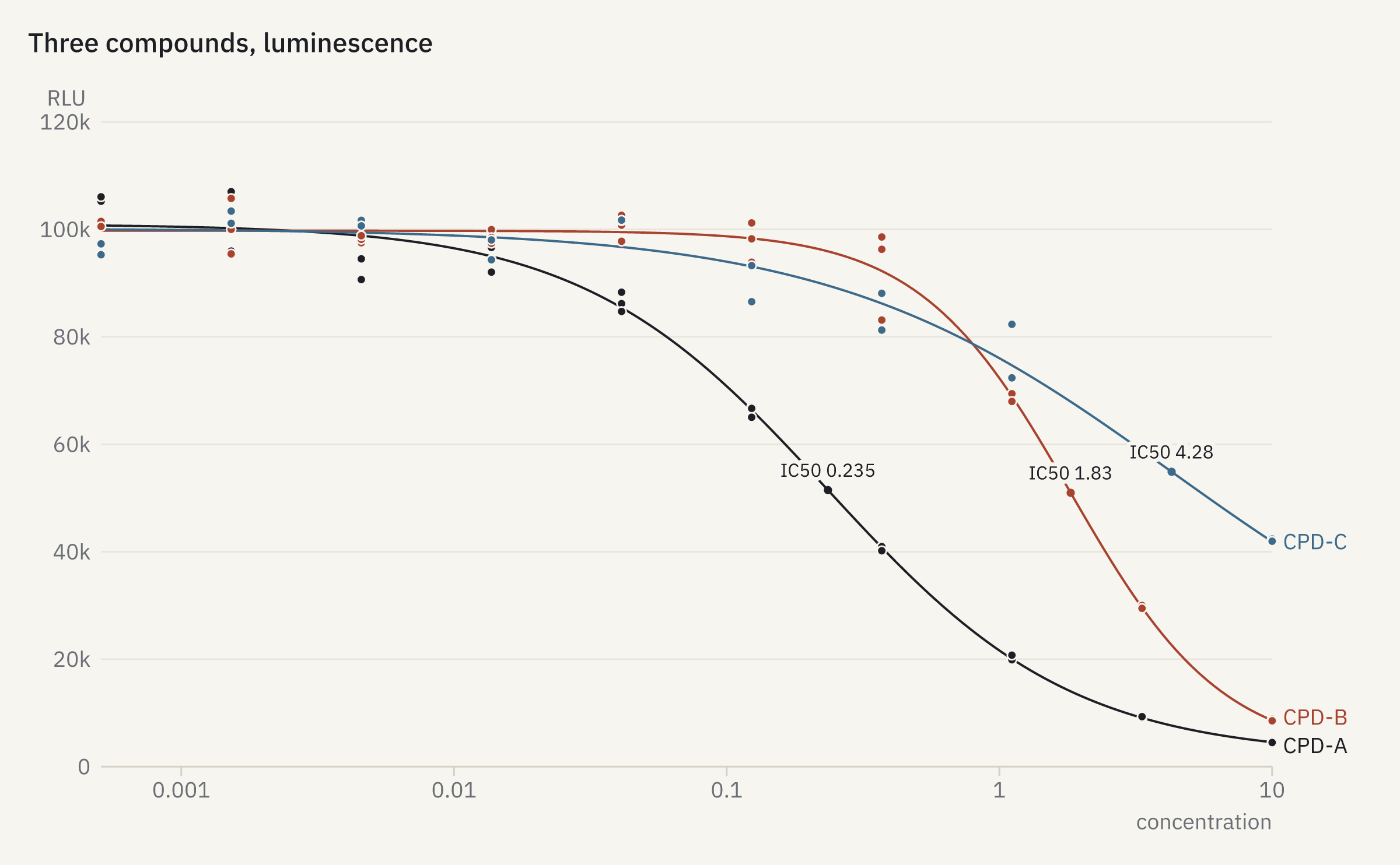
openreadout plot dose-response.json -o dose-response.png{
"title": "Three compounds, luminescence",
"data": {
"file": "assay-synth-dose-response.csv",
"assay": {
"layout": "assay-synth-dose-response-layout.csv"
}
}
}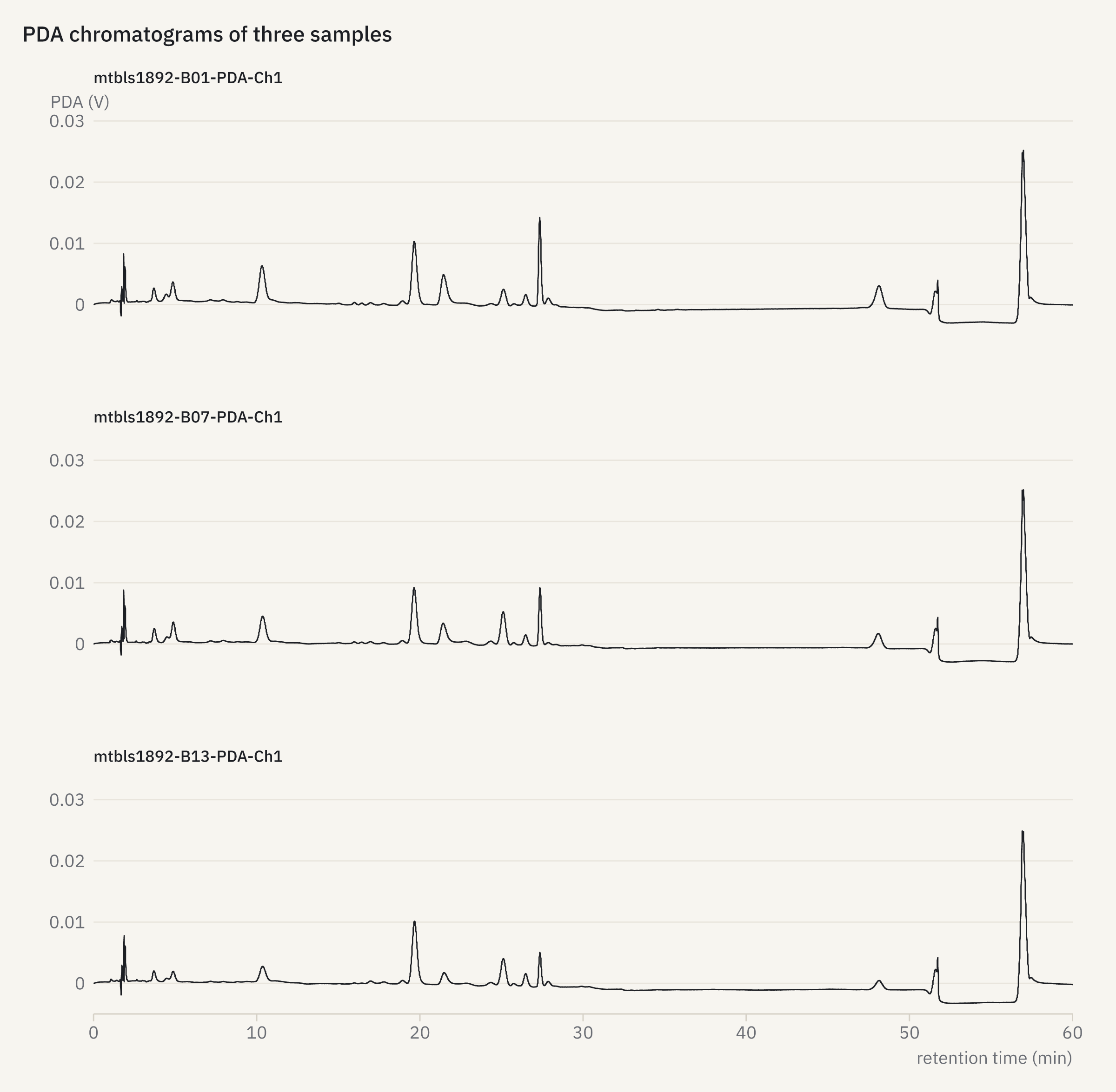
How it was made
openreadout plot chromatograms.json -o chromatograms.png{
"title": "PDA chromatograms of three samples",
"data": {
"file": [
"mtbls1892-B01-PDA-Ch1.CDF",
"mtbls1892-B07-PDA-Ch1.CDF",
"mtbls1892-B13-PDA-Ch1.CDF"
]
},
"facet": "series",
"columns": 1
}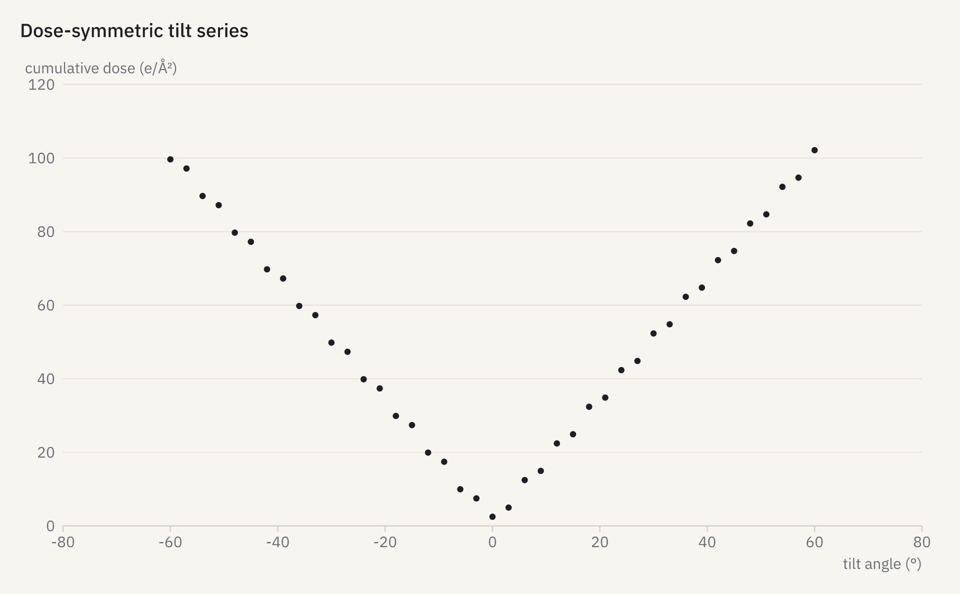
How it was made
openreadout plot tilt-scheme.json -o tilt-scheme.png{
"title": "Dose-symmetric tilt series",
"data": {
"file": "empiar10751-G3_TS_001.mrc.mdoc",
"x": "tilt_angle_deg",
"y": "cumulative_dose_e_per_a2",
"mark": "points"
}
}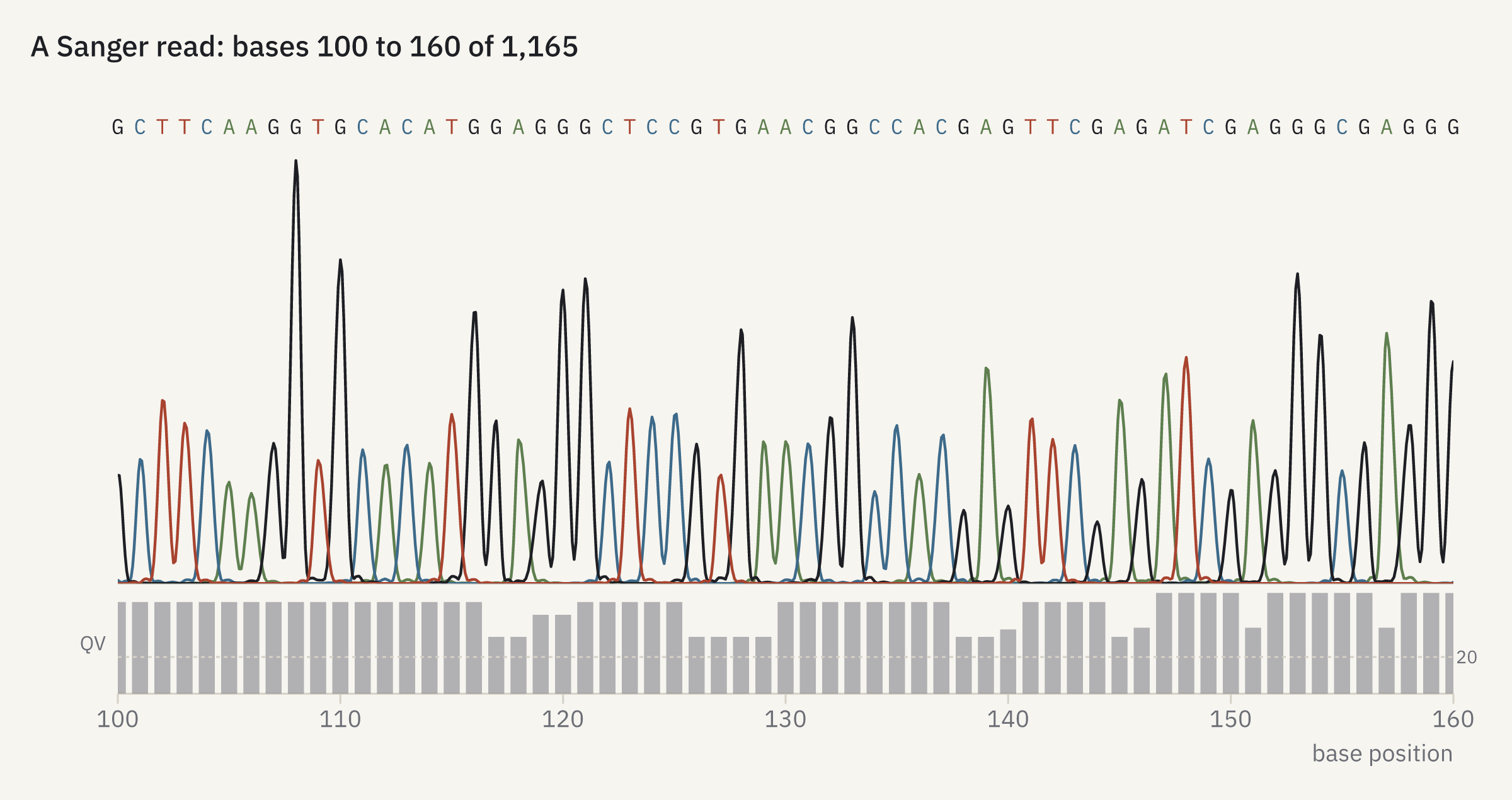
How it was made
openreadout plot sanger-read.json -o sanger-read.png{
"title": "A Sanger read: bases 100 to 160 of 1,165",
"data": {
"file": "abif-biopython-3730.ab1",
"show": "sanger",
"x_range": [
100,
160
]
}
}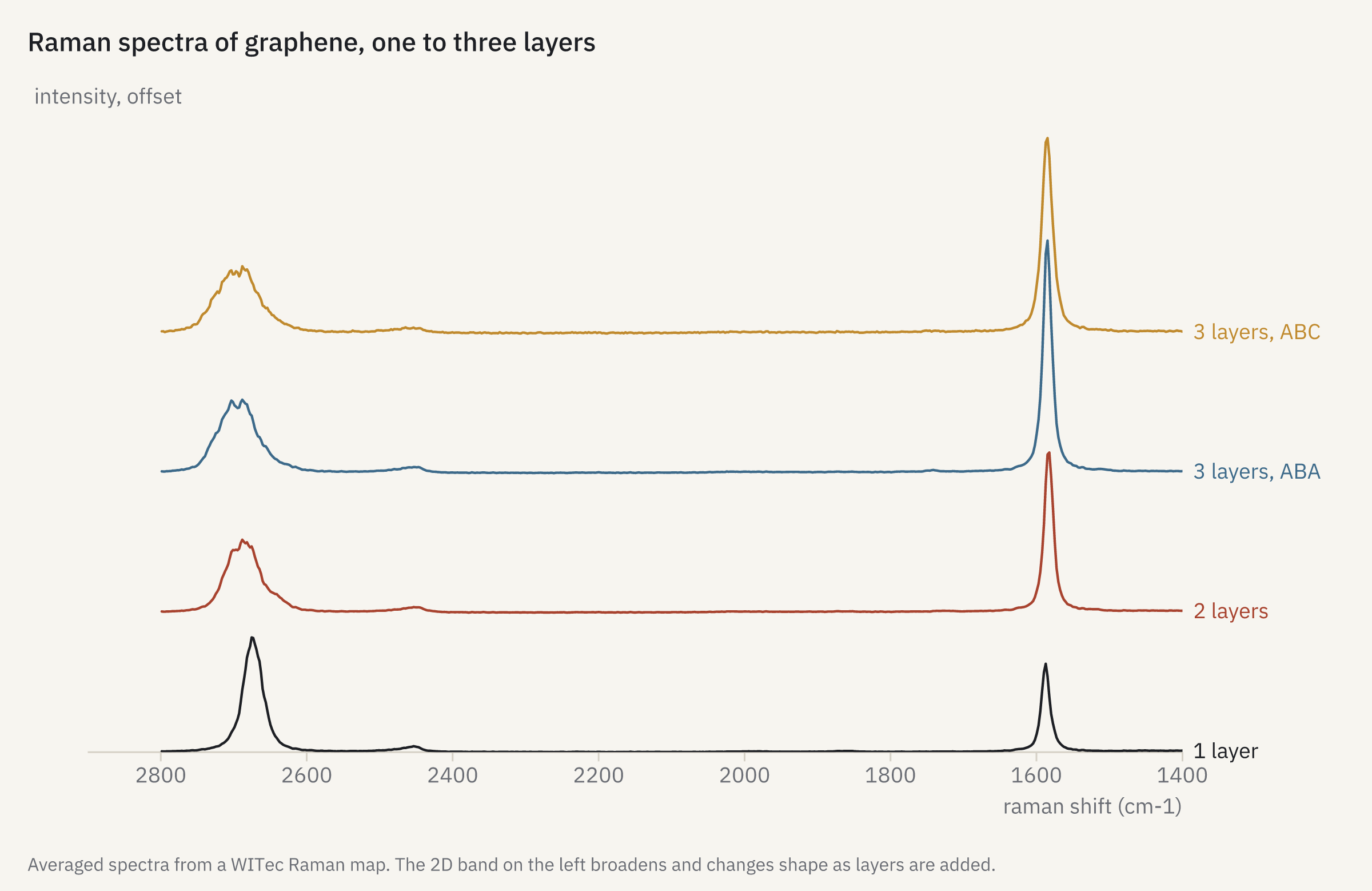
How it was made
openreadout plot raman-graphene.json -o raman-graphene.png{
"title": "Raman spectra of graphene, one to three layers",
"data": [
{
"file": "witio-a-v5-graphene.wip",
"trace": 1,
"label": "1 layer"
},
{
"file": "witio-a-v5-graphene.wip",
"trace": 2,
"label": "2 layers"
},
{
"file": "witio-a-v5-graphene.wip",
"trace": 3,
"label": "3 layers, ABA"
},
{
"file": "witio-a-v5-graphene.wip",
"trace": 4,
"label": "3 layers, ABC"
}
],
"x": {
"range": [
1400,
2900
]
},
"stack": 0.6,
"caption": "Averaged spectra from a WITec Raman map. The 2D band on the left broadens and changes shape as layers are added."
}
How it was made
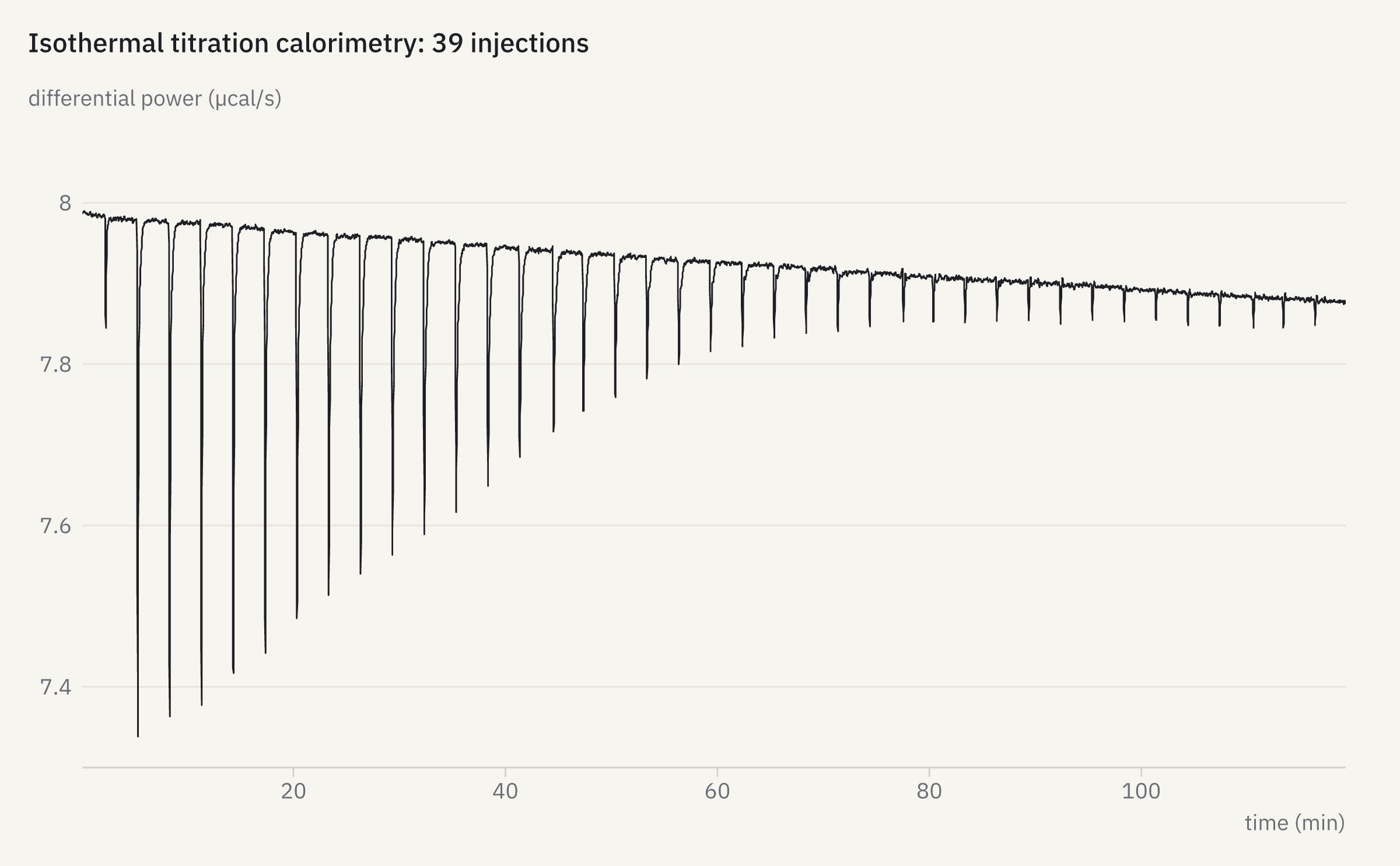
openreadout plot itc-thermogram.json -o itc-thermogram.png{
"title": "Isothermal titration calorimetry: 39 injections",
"data": {
"file": "itc-zenodo6608282-d25-50um.itc",
"channel": 0
}
}
How it was made
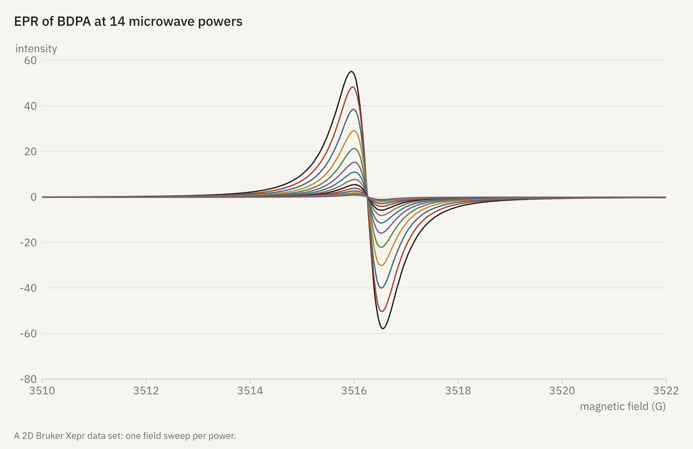
openreadout plot epr-power-series.json -o epr-power-series.png{
"title": "EPR of BDPA at 14 microwave powers",
"data": {
"file": "epr-cwepr-bdpa-2dfieldpower.DSC",
"sweep": [
0,
1,
2,
3,
4,
5,
6,
7,
8,
9,
10,
11,
12,
13
]
},
"x": {
"range": [
3510,
3522
]
},
"legend": "none",
"caption": "A 2D Bruker Xepr data set: one field sweep per power."
}
How it was made
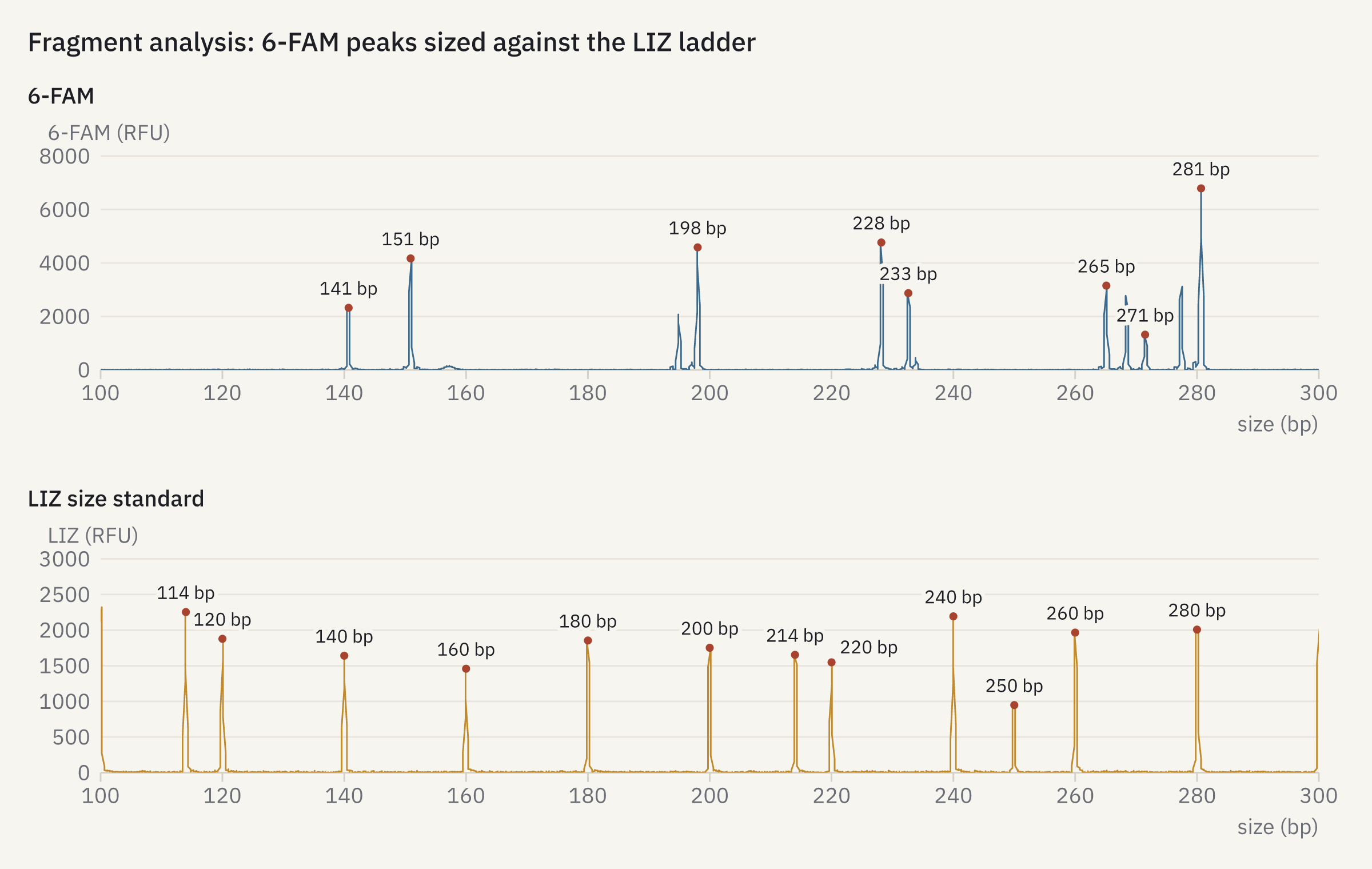
openreadout plot fragment-analysis.json -o fragment-analysis.png{
"title": "Fragment analysis: 6-FAM peaks sized against the LIZ ladder",
"panels": [
{
"title": "6-FAM",
"data": {
"file": "abif-fraggler-multiplex.fsa",
"trace": 0,
"channel": 1,
"peaks": 8,
"color": "blue"
},
"x": {
"range": [
100,
300
]
}
},
{
"title": "LIZ size standard",
"data": {
"file": "abif-fraggler-multiplex.fsa",
"trace": 0,
"channel": 5,
"peaks": 12,
"color": "ochre"
},
"x": {
"range": [
100,
300
]
}
}
],
"columns": 1,
"width": 1200,
"height": 760
}
How it was made
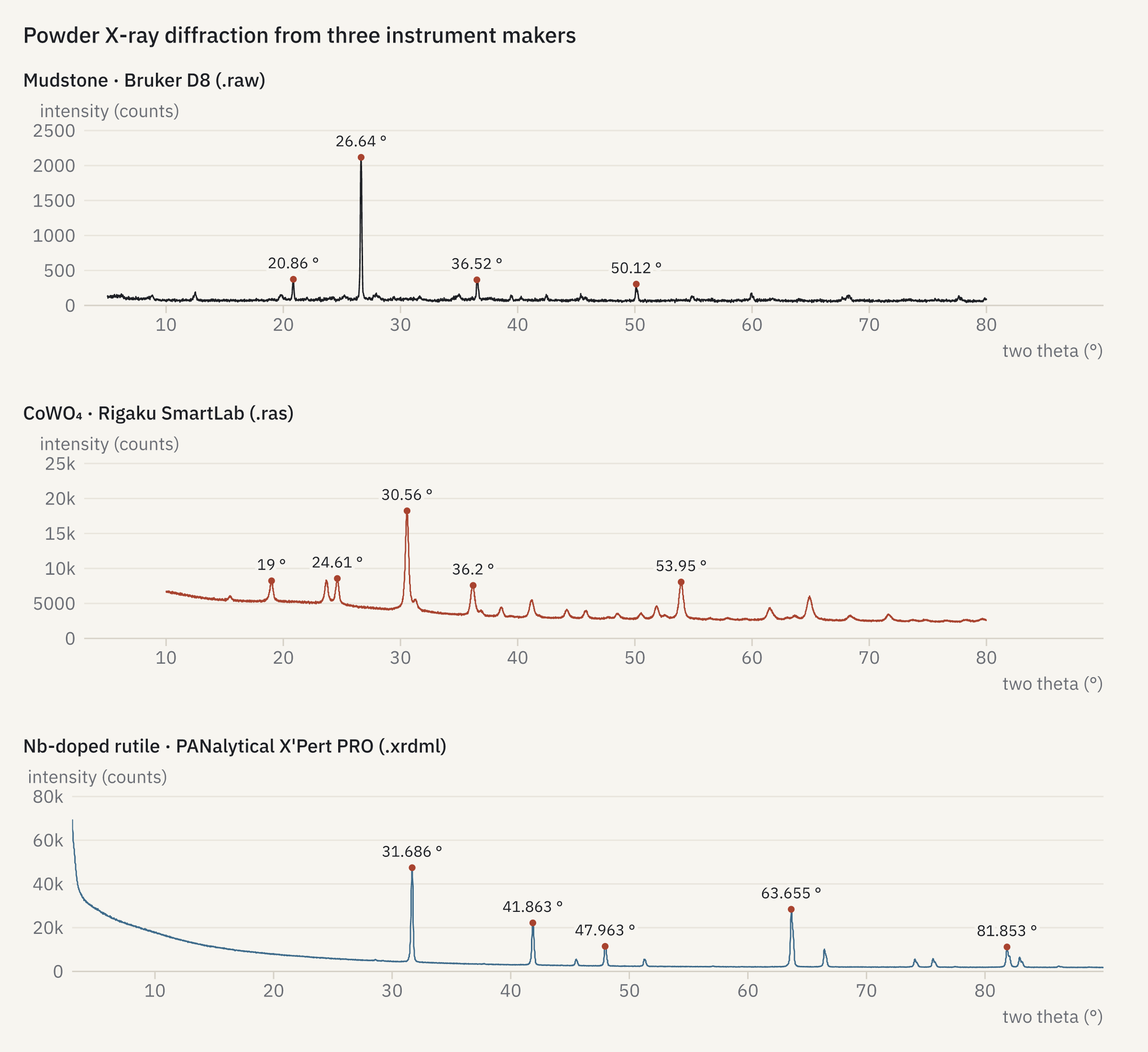
openreadout plot xrd-three-makers.json -o xrd-three-makers.png{
"title": "Powder X-ray diffraction from three instrument makers",
"panels": [
{
"title": "Mudstone · Bruker D8 (.raw)",
"data": {
"file": "xrd-zenodo17012484-raw1-mudstone.raw",
"peaks": 4
}
},
{
"title": "CoWO₄ · Rigaku SmartLab (.ras)",
"data": {
"file": "xrd-zenodo11161891-ras-cowo4.ras",
"peaks": 5,
"color": "accent"
}
},
{
"title": "Nb-doped rutile · PANalytical X'Pert PRO (.xrdml)",
"data": {
"file": "xrd-zenodo5484779-rutile-nb5.xrdml",
"peaks": 5,
"color": "blue"
}
}
],
"columns": 1,
"share": "x",
"width": 1200,
"height": 1100
}
How it was made
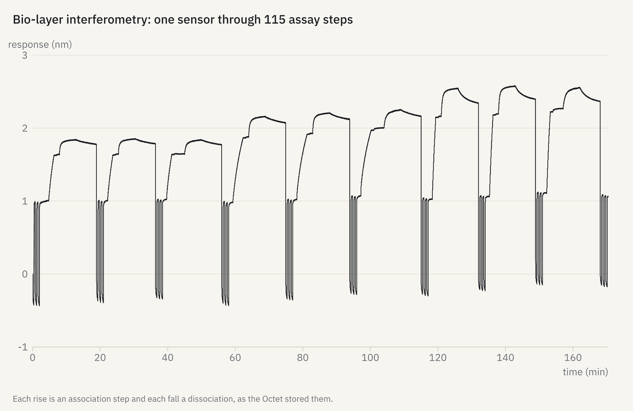
openreadout plot bli-sensor.json -o bli-sensor.png{
"title": "Bio-layer interferometry: one sensor through 115 assay steps",
"data": {
"file": "octet-pykingenie-230309_001.frd",
"channel": 1
},
"caption": "Each rise is an association step and each fall a dissociation, as the Octet stored them."
}
How it was made
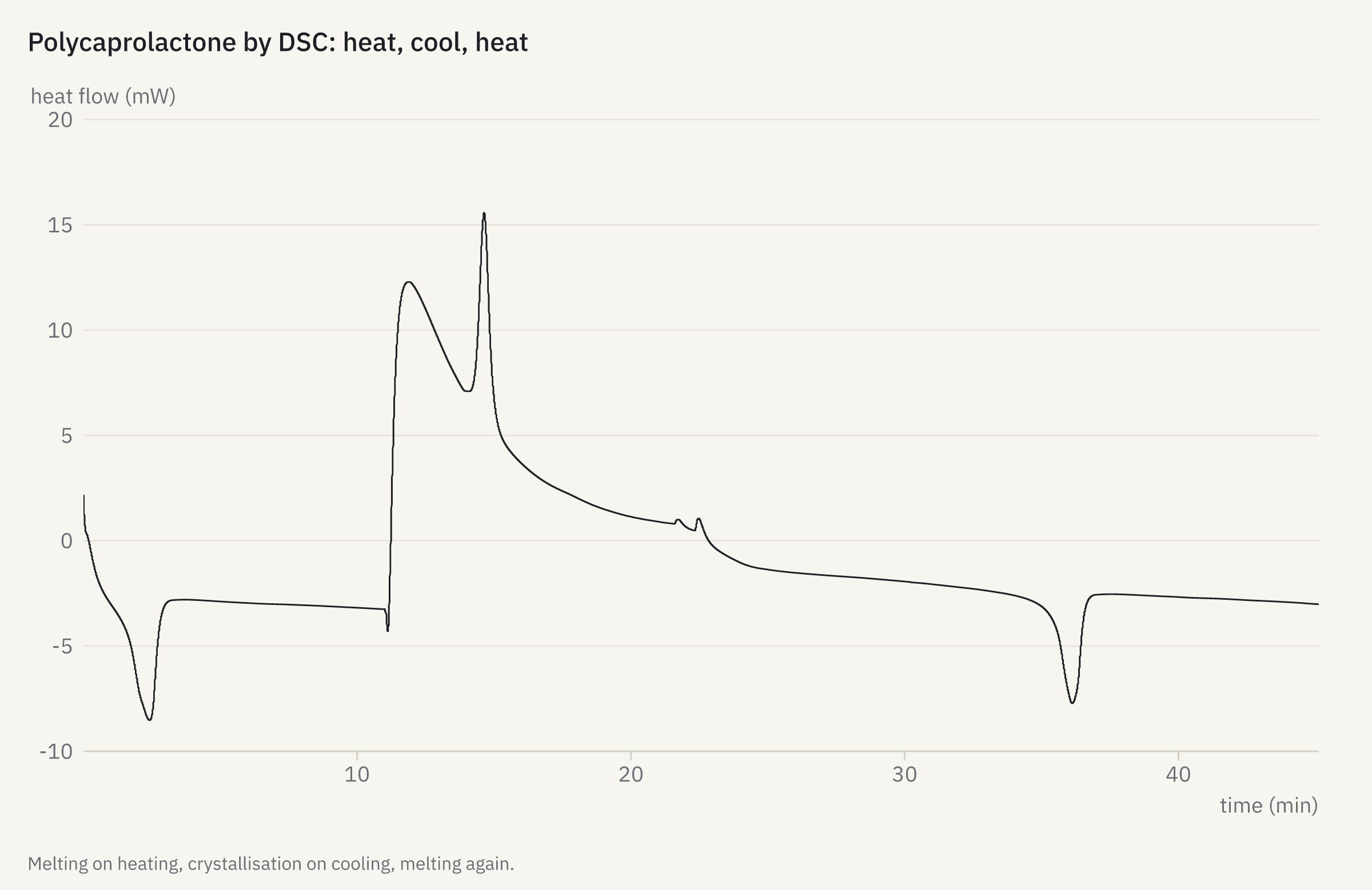
openreadout plot dsc-thermogram.json -o dsc-thermogram.png{
"title": "Polycaprolactone by DSC: heat, cool, heat",
"data": {
"file": "ta-zenodo17293641-pcl-standard.001",
"channel": 2
},
"caption": "Melting on heating, crystallisation on cooling, melting again."
}Make your own
The plot reference lists every key of a figure spec, and the
preview reference every option and annotation. In Python, openreadout.plot() and
File.preview() return pictures that show themselves in Jupyter (Python guide); R has
openreadout_plot() and openreadout_preview() (R guide).
Drawn by OpenReadout 0.4.0 with node book/scripts/gallery.mjs. The files are public: Zenodo, Dryad, figshare, MetaboLights, EMDB, EMPIAR and Image Data Resource records,
the OME sample images, the Cell Painting Gallery, and the test data of pyABF, FlowKit, nmrXiv, Biopython, wit_io, cwepr, Fraggler,
pykingenie and brukerapi, used under their licences (corpus manifest).